Day 49: Time Series & Forecasting
✅ Today you will learn
- What makes time-series data special
- Trend, seasonality and decomposition
- Baselines: naive and seasonal-naive
- ML forecasting with lag and calendar features
- Holt-Winters and time-based validation
🏢 In the real world
Delhi’s schools and hospitals want a 30-day air-quality outlook to plan closures, masks and extra staff. Retailers want next month’s demand, banks next week’s cash withdrawals. All of these are forecasting problems – and the rules are different from normal ML because the future must never leak into the past.
Look at the series
import pandas as pd
import matplotlib.pyplot as plt
w = pd.read_csv("delhi_weather.csv", parse_dates=["date"]).set_index("date").asfreq("D")
print(w.shape, "| missing days:", w["aqi"].isna().sum())
m = w["aqi"].resample("MS").mean()
fig, ax = plt.subplots(figsize=(10, 3.6))
ax.plot(w.index, w["aqi"], color="#cbd5e1", lw=0.7, label="daily")
ax.plot(m.index, m.values, color="#dc2626", marker="o", lw=2, label="monthly mean")
ax.set_title("Delhi AQI 2022–2024: strong yearly seasonality"); ax.legend(); plt.show()
Trend + seasonality + noise
import pandas as pd
import matplotlib.pyplot as plt
from statsmodels.tsa.seasonal import seasonal_decompose
w = pd.read_csv("delhi_weather.csv", parse_dates=["date"]).set_index("date")
weekly = w["aqi"].resample("W").mean()
dec = seasonal_decompose(weekly, model="additive", period=52)
fig = dec.plot(); fig.set_size_inches(10, 6.5); fig.suptitle("Decomposition of weekly AQI", y=1.01)
plt.tight_layout(); plt.show()
print("seasonal swing (max − min):", round(dec.seasonal.max() - dec.seasonal.min()), "AQI points")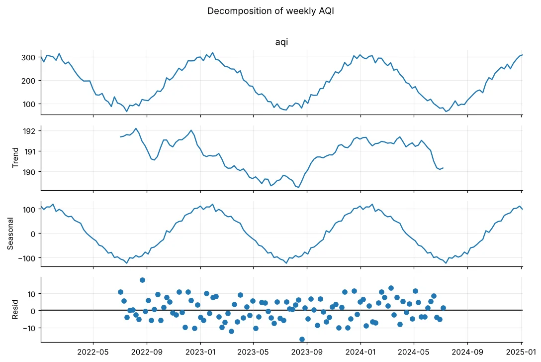
Split by time, never randomly
import pandas as pd
w = pd.read_csv("delhi_weather.csv", parse_dates=["date"]).set_index("date")
train, test = w.loc[:"2023-12-31", "aqi"], w.loc["2024-01-01":, "aqi"]
print("train:", train.index.min().date(), "→", train.index.max().date(), len(train))
print("test :", test.index.min().date(), "→", test.index.max().date(), len(test))With train_test_split, a model could learn from 15 March to predict 14 March – impossible in real life. Always train on the past and test on the future (or use TimeSeriesSplit).
Baselines first
import numpy as np
import pandas as pd
from sklearn.metrics import mean_absolute_error, mean_absolute_percentage_error
w = pd.read_csv("delhi_weather.csv", parse_dates=["date"]).set_index("date")["aqi"]
test = w.loc["2024"]
preds = {"naive (last value of 2023)": pd.Series(w.loc["2023-12-31"], index=test.index),
         "mean of 2022–23": pd.Series(w.loc[:"2023"].mean(), index=test.index),
         "seasonal naive (same day last year)": w.shift(365).loc["2024"]}
for name, p in preds.items():
print(f"{name:36s} MAE {mean_absolute_error(test, p):6.1f} MAPE {mean_absolute_percentage_error(test, p) * 100:5.1f}%")Mean absolute percentage error: “on average we are 18% off”. Easy for managers, but unstable when actual values are near zero (sales of 0 units).
Machine learning with lag features
import numpy as np
import pandas as pd
from sklearn.ensemble import HistGradientBoostingRegressor
from sklearn.metrics import mean_absolute_error
w = pd.read_csv("delhi_weather.csv", parse_dates=["date"]).set_index("date")
f = pd.DataFrame(index=w.index)
f["aqi"] = w["aqi"]
f["lag_365"] = w["aqi"].shift(365)                   # same day last year
f["lag_30"] = w["aqi"].shift(30)                     # a month ago (known 30 days ahead)
f["roll_30_lag_30"] = w["aqi"].shift(30).rolling(30).mean()
f["doy_sin"] = np.sin(2 * np.pi * w.index.dayofyear / 365.25)
f["doy_cos"] = np.cos(2 * np.pi * w.index.dayofyear / 365.25)
f["weekday"] = w.index.dayofweek
f = f.dropna()
tr, te = f.loc[:"2023"], f.loc["2024"]
feats = [c for c in f.columns if c != "aqi"]
model = HistGradientBoostingRegressor(max_iter=300, learning_rate=0.05, random_state=0).fit(tr[feats], tr["aqi"])
pred = pd.Series(model.predict(te[feats]), index=te.index)
print("training rows:", len(tr), "| features:", feats)
print(f"ML forecast MAE {mean_absolute_error(te['aqi'], pred):.1f}")
pred.to_frame("pred").assign(actual=te["aqi"]).to_csv("aqi_forecast_2024.csv")For a 30-day-ahead forecast, yesterday’s AQI is not available – so the shortest lag is 30 days. Matching the lags to the forecast horizon is the time-series version of avoiding leakage.
Holt-Winters exponential smoothing
import pandas as pd
import matplotlib.pyplot as plt
from statsmodels.tsa.holtwinters import ExponentialSmoothing
from sklearn.metrics import mean_absolute_error
w = pd.read_csv("delhi_weather.csv", parse_dates=["date"]).set_index("date")["aqi"]
monthly = w.resample("MS").mean()
train, test = monthly.loc[:"2023"], monthly.loc["2024"]
hw = ExponentialSmoothing(train, trend=None, seasonal="additive", seasonal_periods=12).fit()
fc = hw.forecast(12)
snaive = monthly.shift(12).loc["2024"]
print(f"monthly MAE → Holt-Winters {mean_absolute_error(test, fc):.1f} | seasonal naive {mean_absolute_error(test, snaive):.1f}")
plt.figure(figsize=(10, 3.8))
plt.plot(monthly.index, monthly, color="#64748b", marker="o", label="actual")
plt.plot(fc.index, fc, color="#dc2626", marker="o", ls="--", label="Holt-Winters forecast 2024")
plt.axvspan(test.index.min(), test.index.max(), color="#fee2e2", alpha=0.5)
plt.title("Forecasting 2024 monthly AQI from 2022–23 only"); plt.legend(); plt.show()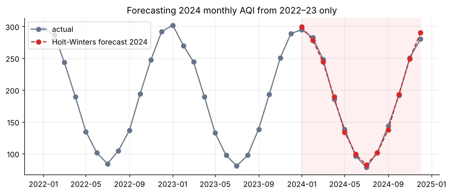
Time-series cross-validation
import numpy as np
from sklearn.model_selection import TimeSeriesSplit
idx = np.arange(12)
for i, (tr, te) in enumerate(TimeSeriesSplit(n_splits=4, test_size=2).split(idx), 1):
print(f"fold {i}: train months {tr.min()}–{tr.max()} → test months {te.tolist()}")| Method | Good for |
|---|---|
| Seasonal naive | Always – the baseline to beat |
| Holt-Winters / ETS | Clear trend + seasonality, few series |
| ARIMA / SARIMA | Classic statistical forecasting, short-term |
| Prophet | Business series with holidays (Diwali!), easy to use |
| ML with lags (boosting) | Many related series, extra features like weather, promotions |
🏅 Job skills unlocked today
Practice tasks
🏋️ Practice – do it yourself
Show solution
import pandas as pd
from statsmodels.tsa.holtwinters import ExponentialSmoothing
from sklearn.metrics import mean_absolute_error
t = pd.read_csv("delhi_weather.csv", parse_dates=["date"]).set_index("date")["avg_temp_c"].resample("MS").mean()
fc = ExponentialSmoothing(t.loc[:"2023"], seasonal="additive", seasonal_periods=12).fit().forecast(12)
print("HW", round(mean_absolute_error(t.loc["2024"], fc), 2), "| seasonal naive", round(mean_absolute_error(t.loc["2024"], t.shift(12).loc["2024"]), 2))Show solution
import pandas as pd
s = pd.read_csv("sales_data.csv", parse_dates=["order_date"]); s["rev"] = s["quantity"] * s["unit_price"] * (1 - s["discount"])
wk = s.set_index("order_date")["rev"].resample("W").sum()
ma = wk.shift(1).rolling(4).mean()
print(pd.DataFrame({"actual": wk, "moving_avg_forecast": ma}).tail(8).round(0))Quick quiz
🧠 Quick Quiz – test yourself
Interview corner
💼 Interview Corner
How is time-series validation different?
Data must be split by time – train on earlier periods, test on later ones – using expanding or rolling windows (TimeSeriesSplit). Features must only use information available at forecast time.
What baselines do you use for forecasting?
Naive (last value), seasonal naive (same period last season) and a moving average. A complex model is only useful if it clearly beats them.
Summary
- Time series = trend + seasonality + noise.
- Split by time; beat naive and seasonal-naive baselines.
- ML with lags matched to the horizon + calendar features works well.
- Holt-Winters is a strong simple seasonal model; report MAE and MAPE.
Day 50: deploy your model – save it with joblib and serve predictions with Streamlit and Flask.