🏆 Major Project – Churn Prediction · Day 59

Day 59: Project 4: Evaluation & Business Impact

⏱ 3.5 hours📶 Major project · Part 4 of 5🎯 100% self-study

Day 59 / 60

✅ Today you will learn

Open the locked test set – once
ROC-AUC, PR-AUC, confusion matrix
Gains & lift: value of calling the top 20%
Pick the call list size by profit, not by 0.5
Explain each prediction and check fairness

🏢 In the real world

The Head of Retention asks three questions before approving the budget: “How good is the model on customers it has never seen? How many people should my team call each month? How much money will we actually save?” Today you answer all three with numbers.

Step 1: the moment of truth

Python

import numpy as np
import pandas as pd

def load_churn(path="telecom_churn.csv"):
    # "None" means no internet plan – stop pandas from turning it into NaN
    df = pd.read_csv(path, keep_default_na=False, na_values=[""])
    df["total_charges"] = df["total_charges"].fillna(df["monthly_charges"] * df["tenure_months"])
    df["churned"] = (df["churn"] == "Yes").astype(int)
    return df

def add_features(df):
    df = df.copy()
    df["tenure_band"] = pd.cut(df["tenure_months"], [0, 6, 12, 24, 48, 72], labels=["0-6", "7-12", "13-24", "25-48", "49-72"]).astype(str)
    df["is_new"] = (df["tenure_months"] <= 6).astype(int)
    df["has_complaint"] = (df["complaints"] > 0).astype(int)
    df["charge_per_gb"] = (df["monthly_charges"] / df["data_usage_gb"].clip(lower=1)).round(2)
    df["avg_monthly_paid"] = (df["total_charges"] / df["tenure_months"]).round(1)
    df["monthly_no_support"] = ((df["contract"] == "Monthly") & (df["tech_support"] == "No")).astype(int)
    return df

# original columns – the champion model uses these
NUM = ["senior_citizen", "tenure_months", "monthly_charges", "total_charges", "complaints", "data_usage_gb"]
CAT = ["gender", "contract", "internet_service", "tech_support", "payment_method"]
# original + engineered columns (tested on Day 58)
NUM_ALL = NUM + ["is_new", "has_complaint", "charge_per_gb", "avg_monthly_paid", "monthly_no_support"]
CAT_ALL = CAT + ["tenure_band"]

from sklearn.compose import ColumnTransformer
from sklearn.preprocessing import OneHotEncoder, StandardScaler
from sklearn.pipeline import Pipeline
from sklearn.linear_model import LogisticRegression
from sklearn.model_selection import train_test_split

df = add_features(load_churn())
X, y = df[NUM_ALL + CAT_ALL], df["churned"]          # keep all columns; each model picks what it needs
X_dev, X_test, y_dev, y_test = train_test_split(X, y, test_size=0.2, random_state=2025, stratify=y)

def make_model(C=0.1, num=NUM, cat=CAT):
    pre = ColumnTransformer([("num", StandardScaler(), num), ("cat", OneHotEncoder(handle_unknown="ignore"), cat)])
    return Pipeline([("prep", pre), ("clf", LogisticRegression(C=C, max_iter=5000))])

model = make_model().fit(X_dev, y_dev)                        # champion: original columns, C = 0.1
p_test = model.predict_proba(X_test)[:, 1]

from sklearn.metrics import roc_auc_score, average_precision_score, classification_report
print(f"TEST ROC-AUC = {roc_auc_score(y_test, p_test):.3f}   (CV on dev was ≈ 0.82)")
print(f"TEST PR-AUC  = {average_precision_score(y_test, p_test):.3f}   (random = {y_test.mean():.3f})")
print(classification_report(y_test, (p_test >= 0.5).astype(int), target_names=["stays", "churns"], digits=3))

TEST ROC-AUC = 0.832 (CV on dev was ≈ 0.82) TEST PR-AUC = 0.679 (random = 0.292) precision recall f1-score support stays 0.830 0.918 0.872 425 churns 0.731 0.543 0.623 175 accuracy 0.808 600 macro avg 0.780 0.730 0.747 600 weighted avg 0.801 0.808 0.799 600

✅ No surprise is good news

The test AUC is close to the cross-validation estimate. That means our process was honest: no leakage, no over-tuning. A big drop would have been a warning to investigate before going live.

Python

import numpy as np
import pandas as pd

def load_churn(path="telecom_churn.csv"):
    # "None" means no internet plan – stop pandas from turning it into NaN
    df = pd.read_csv(path, keep_default_na=False, na_values=[""])
    df["total_charges"] = df["total_charges"].fillna(df["monthly_charges"] * df["tenure_months"])
    df["churned"] = (df["churn"] == "Yes").astype(int)
    return df

def add_features(df):
    df = df.copy()
    df["tenure_band"] = pd.cut(df["tenure_months"], [0, 6, 12, 24, 48, 72], labels=["0-6", "7-12", "13-24", "25-48", "49-72"]).astype(str)
    df["is_new"] = (df["tenure_months"] <= 6).astype(int)
    df["has_complaint"] = (df["complaints"] > 0).astype(int)
    df["charge_per_gb"] = (df["monthly_charges"] / df["data_usage_gb"].clip(lower=1)).round(2)
    df["avg_monthly_paid"] = (df["total_charges"] / df["tenure_months"]).round(1)
    df["monthly_no_support"] = ((df["contract"] == "Monthly") & (df["tech_support"] == "No")).astype(int)
    return df

# original columns – the champion model uses these
NUM = ["senior_citizen", "tenure_months", "monthly_charges", "total_charges", "complaints", "data_usage_gb"]
CAT = ["gender", "contract", "internet_service", "tech_support", "payment_method"]
# original + engineered columns (tested on Day 58)
NUM_ALL = NUM + ["is_new", "has_complaint", "charge_per_gb", "avg_monthly_paid", "monthly_no_support"]
CAT_ALL = CAT + ["tenure_band"]

from sklearn.compose import ColumnTransformer
from sklearn.preprocessing import OneHotEncoder, StandardScaler
from sklearn.pipeline import Pipeline
from sklearn.linear_model import LogisticRegression
from sklearn.model_selection import train_test_split

df = add_features(load_churn())
X, y = df[NUM_ALL + CAT_ALL], df["churned"]          # keep all columns; each model picks what it needs
X_dev, X_test, y_dev, y_test = train_test_split(X, y, test_size=0.2, random_state=2025, stratify=y)

def make_model(C=0.1, num=NUM, cat=CAT):
    pre = ColumnTransformer([("num", StandardScaler(), num), ("cat", OneHotEncoder(handle_unknown="ignore"), cat)])
    return Pipeline([("prep", pre), ("clf", LogisticRegression(C=C, max_iter=5000))])

model = make_model().fit(X_dev, y_dev)                        # champion: original columns, C = 0.1
p_test = model.predict_proba(X_test)[:, 1]

import matplotlib.pyplot as plt
from sklearn.metrics import RocCurveDisplay, PrecisionRecallDisplay, ConfusionMatrixDisplay
fig, ax = plt.subplots(1, 3, figsize=(15, 4.2))
RocCurveDisplay.from_predictions(y_test, p_test, ax=ax[0], name="champion"); ax[0].plot([0, 1], [0, 1], "k:"); ax[0].set_title("ROC curve (test)")
PrecisionRecallDisplay.from_predictions(y_test, p_test, ax=ax[1], name="champion"); ax[1].axhline(y_test.mean(), color="k", ls=":"); ax[1].set_title("Precision–recall (test)")
ConfusionMatrixDisplay.from_predictions(y_test, (p_test >= 0.5).astype(int), display_labels=["stays", "churns"], cmap="Blues", colorbar=False, ax=ax[2])
ax[2].set_title("Confusion matrix at 0.5")
plt.tight_layout(); plt.show()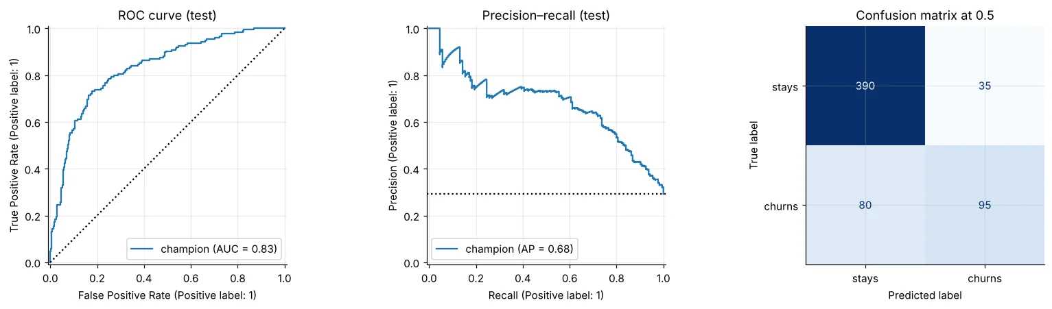

ROC curve, precision-recall curve and confusion matrix on the test set — Dotted lines = random guessing. The model is clearly better – but 0.5 is not necessarily the right cut-off.

Step 2: gains and lift – what calling the top X% achieves

Python

import numpy as np
import pandas as pd

def load_churn(path="telecom_churn.csv"):
    # "None" means no internet plan – stop pandas from turning it into NaN
    df = pd.read_csv(path, keep_default_na=False, na_values=[""])
    df["total_charges"] = df["total_charges"].fillna(df["monthly_charges"] * df["tenure_months"])
    df["churned"] = (df["churn"] == "Yes").astype(int)
    return df

def add_features(df):
    df = df.copy()
    df["tenure_band"] = pd.cut(df["tenure_months"], [0, 6, 12, 24, 48, 72], labels=["0-6", "7-12", "13-24", "25-48", "49-72"]).astype(str)
    df["is_new"] = (df["tenure_months"] <= 6).astype(int)
    df["has_complaint"] = (df["complaints"] > 0).astype(int)
    df["charge_per_gb"] = (df["monthly_charges"] / df["data_usage_gb"].clip(lower=1)).round(2)
    df["avg_monthly_paid"] = (df["total_charges"] / df["tenure_months"]).round(1)
    df["monthly_no_support"] = ((df["contract"] == "Monthly") & (df["tech_support"] == "No")).astype(int)
    return df

# original columns – the champion model uses these
NUM = ["senior_citizen", "tenure_months", "monthly_charges", "total_charges", "complaints", "data_usage_gb"]
CAT = ["gender", "contract", "internet_service", "tech_support", "payment_method"]
# original + engineered columns (tested on Day 58)
NUM_ALL = NUM + ["is_new", "has_complaint", "charge_per_gb", "avg_monthly_paid", "monthly_no_support"]
CAT_ALL = CAT + ["tenure_band"]

from sklearn.compose import ColumnTransformer
from sklearn.preprocessing import OneHotEncoder, StandardScaler
from sklearn.pipeline import Pipeline
from sklearn.linear_model import LogisticRegression
from sklearn.model_selection import train_test_split

df = add_features(load_churn())
X, y = df[NUM_ALL + CAT_ALL], df["churned"]          # keep all columns; each model picks what it needs
X_dev, X_test, y_dev, y_test = train_test_split(X, y, test_size=0.2, random_state=2025, stratify=y)

def make_model(C=0.1, num=NUM, cat=CAT):
    pre = ColumnTransformer([("num", StandardScaler(), num), ("cat", OneHotEncoder(handle_unknown="ignore"), cat)])
    return Pipeline([("prep", pre), ("clf", LogisticRegression(C=C, max_iter=5000))])

model = make_model().fit(X_dev, y_dev)                        # champion: original columns, C = 0.1
p_test = model.predict_proba(X_test)[:, 1]

import matplotlib.pyplot as plt
t = pd.DataFrame({"y": y_test.values, "p": p_test}).sort_values("p", ascending=False).reset_index(drop=True)
t["decile"] = t.index // (len(t) // 10) + 1
dec = t.groupby("decile").agg(customers=("y", "size"), churners=("y", "sum"), churn_rate=("y", "mean"))
dec["cum_capture_%"] = (dec["churners"].cumsum() / dec["churners"].sum() * 100).round(1)
dec["lift"] = (dec["churn_rate"] / t["y"].mean()).round(2)
print(dec.round(3).to_string())
fig, ax = plt.subplots(1, 2, figsize=(12, 4))
pct = np.arange(0, 101, 10)
ax[0].plot(pct, [0] + list(dec["cum_capture_%"]), marker="o", color="#4f46e5", label="model"); ax[0].plot([0, 100], [0, 100], "k:", label="random")
ax[0].set_xlabel("% of customers called (highest risk first)"); ax[0].set_ylabel("% of churners reached"); ax[0].set_title("Cumulative gains"); ax[0].legend()
ax[1].bar(dec.index, dec["lift"], color=["#dc2626" if l > 1.5 else "#94a3b8" for l in dec["lift"]]); ax[1].axhline(1, color="k", ls=":")
ax[1].set_xlabel("risk decile (1 = highest)"); ax[1].set_title("Lift per decile")
plt.tight_layout(); plt.show()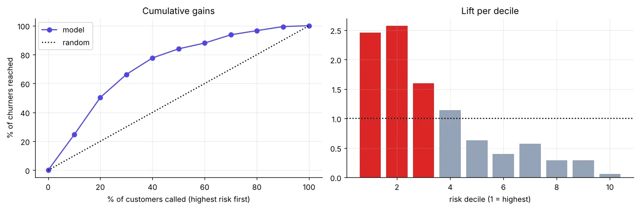

customers churners churn_rate cum_capture_% lift decile 1 60 43 0.717 24.6 2.46 2 60 45 0.750 50.3 2.57 3 60 28 0.467 66.3 1.60 4 60 20 0.333 77.7 1.14 5 60 11 0.183 84.0 0.63 6 60 7 0.117 88.0 0.40 7 60 10 0.167 93.7 0.57 8 60 5 0.083 96.6 0.29 9 60 5 0.083 99.4 0.29 10 60 1 0.017 100.0 0.06

Cumulative gains curve and lift by decile for the churn model — Calling the top 20% reaches a much larger share of churners than random calling.

Step 3: how many customers to call? Let profit decide

Using the assumptions from Day 56: each call costs ₹40; a reached churner is saved with 30% probability and is worth one more year of their bill minus the ₹600 offer; but half of the non-churners we call also accept the discount – ₹600 wasted on people who would have stayed. We choose the list size on the development out-of-fold predictions, then confirm it on the test set.

Python

import numpy as np
import pandas as pd

def load_churn(path="telecom_churn.csv"):
    # "None" means no internet plan – stop pandas from turning it into NaN
    df = pd.read_csv(path, keep_default_na=False, na_values=[""])
    df["total_charges"] = df["total_charges"].fillna(df["monthly_charges"] * df["tenure_months"])
    df["churned"] = (df["churn"] == "Yes").astype(int)
    return df

def add_features(df):
    df = df.copy()
    df["tenure_band"] = pd.cut(df["tenure_months"], [0, 6, 12, 24, 48, 72], labels=["0-6", "7-12", "13-24", "25-48", "49-72"]).astype(str)
    df["is_new"] = (df["tenure_months"] <= 6).astype(int)
    df["has_complaint"] = (df["complaints"] > 0).astype(int)
    df["charge_per_gb"] = (df["monthly_charges"] / df["data_usage_gb"].clip(lower=1)).round(2)
    df["avg_monthly_paid"] = (df["total_charges"] / df["tenure_months"]).round(1)
    df["monthly_no_support"] = ((df["contract"] == "Monthly") & (df["tech_support"] == "No")).astype(int)
    return df

# original columns – the champion model uses these
NUM = ["senior_citizen", "tenure_months", "monthly_charges", "total_charges", "complaints", "data_usage_gb"]
CAT = ["gender", "contract", "internet_service", "tech_support", "payment_method"]
# original + engineered columns (tested on Day 58)
NUM_ALL = NUM + ["is_new", "has_complaint", "charge_per_gb", "avg_monthly_paid", "monthly_no_support"]
CAT_ALL = CAT + ["tenure_band"]

from sklearn.compose import ColumnTransformer
from sklearn.preprocessing import OneHotEncoder, StandardScaler
from sklearn.pipeline import Pipeline
from sklearn.linear_model import LogisticRegression
from sklearn.model_selection import train_test_split

df = add_features(load_churn())
X, y = df[NUM_ALL + CAT_ALL], df["churned"]          # keep all columns; each model picks what it needs
X_dev, X_test, y_dev, y_test = train_test_split(X, y, test_size=0.2, random_state=2025, stratify=y)

def make_model(C=0.1, num=NUM, cat=CAT):
    pre = ColumnTransformer([("num", StandardScaler(), num), ("cat", OneHotEncoder(handle_unknown="ignore"), cat)])
    return Pipeline([("prep", pre), ("clf", LogisticRegression(C=C, max_iter=5000))])

import matplotlib.pyplot as plt
from sklearn.model_selection import cross_val_predict, StratifiedKFold
CALL, SAVE_RATE, OFFER, STAYER_ACCEPT = 40, 0.30, 600, 0.5
oof = cross_val_predict(make_model(), X_dev, y_dev, cv=StratifiedKFold(5, shuffle=True, random_state=0), method="predict_proba")[:, 1]
d = pd.DataFrame({"y": y_dev.values, "p": oof, "bill": X_dev["monthly_charges"].values}).sort_values("p", ascending=False)
d["value"] = (d["y"] * SAVE_RATE * (d["bill"] * 12 - OFFER)            # churner saved: one more year minus offer
              - (1 - d["y"]) * STAYER_ACCEPT * OFFER - CALL)           # stayer takes the discount anyway; every call costs ₹40
d["cum_profit"] = d["value"].cumsum()
best_n = int(d["cum_profit"].values.argmax()) + 1
share = best_n / len(d)
print(f"Most profitable list on dev: top {best_n} of {len(d)} customers ({share:.0%}), probability cut-off ≈ {d['p'].iloc[best_n - 1]:.2f}")
plt.figure(figsize=(9, 3.8))
plt.plot(np.arange(1, len(d) + 1) / len(d) * 100, d["cum_profit"] / 1e5, color="#16a34a")
plt.axvline(share * 100, color="#dc2626", ls="--", label=f"best: call top {share:.0%}"); plt.axvline(20, color="#4f46e5", ls=":", label="capacity ≈ 20%")
plt.xlabel("% of customers called"); plt.ylabel("expected net ₹ lakh"); plt.title("Expected profit curve (development data)"); plt.legend()
plt.show()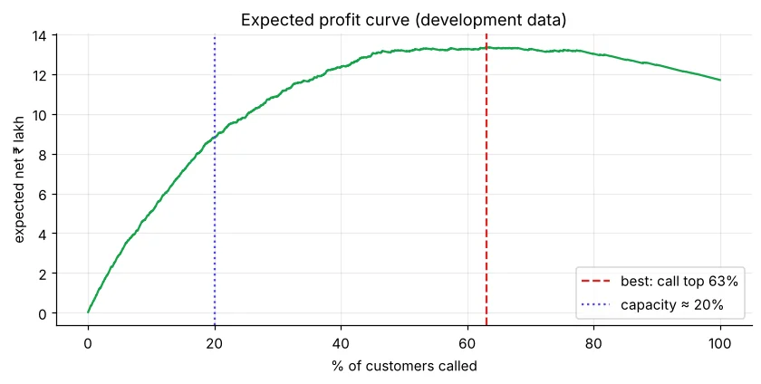

Most profitable list on dev: top 1513 of 2400 customers (63%), probability cut-off ≈ 0.16

Expected profit curve versus percentage of customers called — Profit rises while calls reach likely churners, peaks, then falls as we call people who would stay anyway.

🧠 Profit vs capacity

The profit-maximising list may be larger than the team can call. Then the rule is simple: call the highest-risk customers until capacity runs out – the gains chart tells you exactly what you get for that capacity. If the optimum is much larger than capacity, that is an argument to hire more agents.

Python

import numpy as np
import pandas as pd

def load_churn(path="telecom_churn.csv"):
    # "None" means no internet plan – stop pandas from turning it into NaN
    df = pd.read_csv(path, keep_default_na=False, na_values=[""])
    df["total_charges"] = df["total_charges"].fillna(df["monthly_charges"] * df["tenure_months"])
    df["churned"] = (df["churn"] == "Yes").astype(int)
    return df

def add_features(df):
    df = df.copy()
    df["tenure_band"] = pd.cut(df["tenure_months"], [0, 6, 12, 24, 48, 72], labels=["0-6", "7-12", "13-24", "25-48", "49-72"]).astype(str)
    df["is_new"] = (df["tenure_months"] <= 6).astype(int)
    df["has_complaint"] = (df["complaints"] > 0).astype(int)
    df["charge_per_gb"] = (df["monthly_charges"] / df["data_usage_gb"].clip(lower=1)).round(2)
    df["avg_monthly_paid"] = (df["total_charges"] / df["tenure_months"]).round(1)
    df["monthly_no_support"] = ((df["contract"] == "Monthly") & (df["tech_support"] == "No")).astype(int)
    return df

# original columns – the champion model uses these
NUM = ["senior_citizen", "tenure_months", "monthly_charges", "total_charges", "complaints", "data_usage_gb"]
CAT = ["gender", "contract", "internet_service", "tech_support", "payment_method"]
# original + engineered columns (tested on Day 58)
NUM_ALL = NUM + ["is_new", "has_complaint", "charge_per_gb", "avg_monthly_paid", "monthly_no_support"]
CAT_ALL = CAT + ["tenure_band"]

from sklearn.compose import ColumnTransformer
from sklearn.preprocessing import OneHotEncoder, StandardScaler
from sklearn.pipeline import Pipeline
from sklearn.linear_model import LogisticRegression
from sklearn.model_selection import train_test_split

df = add_features(load_churn())
X, y = df[NUM_ALL + CAT_ALL], df["churned"]          # keep all columns; each model picks what it needs
X_dev, X_test, y_dev, y_test = train_test_split(X, y, test_size=0.2, random_state=2025, stratify=y)

def make_model(C=0.1, num=NUM, cat=CAT):
    pre = ColumnTransformer([("num", StandardScaler(), num), ("cat", OneHotEncoder(handle_unknown="ignore"), cat)])
    return Pipeline([("prep", pre), ("clf", LogisticRegression(C=C, max_iter=5000))])

model = make_model().fit(X_dev, y_dev)                        # champion: original columns, C = 0.1
p_test = model.predict_proba(X_test)[:, 1]

CALL, SAVE_RATE, OFFER, STAYER_ACCEPT, CAPACITY_SHARE = 40, 0.30, 600, 0.5, 0.20
t = pd.DataFrame({"y": y_test.values, "p": p_test, "bill": X_test["monthly_charges"].values}).sort_values("p", ascending=False)
k = int(len(t) * CAPACITY_SHARE)
top, rnd = t.head(k), t.sample(k, random_state=0)
def impact(g):
    saved = g["y"].sum() * SAVE_RATE
    revenue = (g["y"] * g["bill"] * 12).sum() * SAVE_RATE
    wasted = (1 - g["y"]).sum() * STAYER_ACCEPT * OFFER    # discounts given to customers who would stay
    cost = len(g) * CALL + saved * OFFER + wasted
    return g["y"].sum(), saved, revenue - cost
for name, g in [("model top 20%", top), ("random 20%", rnd)]:
    reached, saved, net = impact(g)
    print(f"{name:14s} calls {len(g)} | churners reached {reached:3d} | saved ≈ {saved:4.0f} | net ₹{net / 1e5:5.2f} lakh")
r_m, _, n_m = impact(top); r_r, _, n_r = impact(rnd)
print(f"\nModel reaches {r_m / r_r:.1f}× more churners than random calling.")
scale = 3000 / len(t)                                   # test = 20% of the customer base
print(f"Scaled to the full base each cycle: ≈ ₹{n_m * scale / 1e5:.1f} lakh net vs ₹{n_r * scale / 1e5:.1f} lakh for random calling")

Step 4: can we trust the probabilities?

Python

import numpy as np
import pandas as pd

def load_churn(path="telecom_churn.csv"):
    # "None" means no internet plan – stop pandas from turning it into NaN
    df = pd.read_csv(path, keep_default_na=False, na_values=[""])
    df["total_charges"] = df["total_charges"].fillna(df["monthly_charges"] * df["tenure_months"])
    df["churned"] = (df["churn"] == "Yes").astype(int)
    return df

def add_features(df):
    df = df.copy()
    df["tenure_band"] = pd.cut(df["tenure_months"], [0, 6, 12, 24, 48, 72], labels=["0-6", "7-12", "13-24", "25-48", "49-72"]).astype(str)
    df["is_new"] = (df["tenure_months"] <= 6).astype(int)
    df["has_complaint"] = (df["complaints"] > 0).astype(int)
    df["charge_per_gb"] = (df["monthly_charges"] / df["data_usage_gb"].clip(lower=1)).round(2)
    df["avg_monthly_paid"] = (df["total_charges"] / df["tenure_months"]).round(1)
    df["monthly_no_support"] = ((df["contract"] == "Monthly") & (df["tech_support"] == "No")).astype(int)
    return df

# original columns – the champion model uses these
NUM = ["senior_citizen", "tenure_months", "monthly_charges", "total_charges", "complaints", "data_usage_gb"]
CAT = ["gender", "contract", "internet_service", "tech_support", "payment_method"]
# original + engineered columns (tested on Day 58)
NUM_ALL = NUM + ["is_new", "has_complaint", "charge_per_gb", "avg_monthly_paid", "monthly_no_support"]
CAT_ALL = CAT + ["tenure_band"]

from sklearn.compose import ColumnTransformer
from sklearn.preprocessing import OneHotEncoder, StandardScaler
from sklearn.pipeline import Pipeline
from sklearn.linear_model import LogisticRegression
from sklearn.model_selection import train_test_split

df = add_features(load_churn())
X, y = df[NUM_ALL + CAT_ALL], df["churned"]          # keep all columns; each model picks what it needs
X_dev, X_test, y_dev, y_test = train_test_split(X, y, test_size=0.2, random_state=2025, stratify=y)

def make_model(C=0.1, num=NUM, cat=CAT):
    pre = ColumnTransformer([("num", StandardScaler(), num), ("cat", OneHotEncoder(handle_unknown="ignore"), cat)])
    return Pipeline([("prep", pre), ("clf", LogisticRegression(C=C, max_iter=5000))])

model = make_model().fit(X_dev, y_dev)                        # champion: original columns, C = 0.1
p_test = model.predict_proba(X_test)[:, 1]

import matplotlib.pyplot as plt
from sklearn.calibration import calibration_curve
frac, mean_pred = calibration_curve(y_test, p_test, n_bins=8, strategy="quantile")
plt.figure(figsize=(5.2, 4.6))
plt.plot(mean_pred, frac, marker="o", color="#4f46e5", label="champion"); plt.plot([0, 1], [0, 1], "k:", label="perfect")
plt.xlabel("predicted churn probability"); plt.ylabel("actual churn rate"); plt.title("Calibration (test set)"); plt.legend()
plt.show()
print(pd.DataFrame({"predicted": mean_pred.round(2), "actual": frac.round(2)}).to_string(index=False))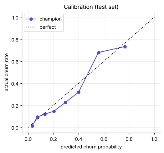

predicted actual 0.03 0.01 0.07 0.09 0.13 0.12 0.20 0.15 0.30 0.23 0.40 0.32 0.56 0.68 0.77 0.73

Calibration curve of predicted versus actual churn — Points near the diagonal mean “70% risk” really behaves like ~70% – important for ₹ forecasts.

Step 5: explain the model – and each customer

Python

import numpy as np
import pandas as pd

def load_churn(path="telecom_churn.csv"):
    # "None" means no internet plan – stop pandas from turning it into NaN
    df = pd.read_csv(path, keep_default_na=False, na_values=[""])
    df["total_charges"] = df["total_charges"].fillna(df["monthly_charges"] * df["tenure_months"])
    df["churned"] = (df["churn"] == "Yes").astype(int)
    return df

def add_features(df):
    df = df.copy()
    df["tenure_band"] = pd.cut(df["tenure_months"], [0, 6, 12, 24, 48, 72], labels=["0-6", "7-12", "13-24", "25-48", "49-72"]).astype(str)
    df["is_new"] = (df["tenure_months"] <= 6).astype(int)
    df["has_complaint"] = (df["complaints"] > 0).astype(int)
    df["charge_per_gb"] = (df["monthly_charges"] / df["data_usage_gb"].clip(lower=1)).round(2)
    df["avg_monthly_paid"] = (df["total_charges"] / df["tenure_months"]).round(1)
    df["monthly_no_support"] = ((df["contract"] == "Monthly") & (df["tech_support"] == "No")).astype(int)
    return df

# original columns – the champion model uses these
NUM = ["senior_citizen", "tenure_months", "monthly_charges", "total_charges", "complaints", "data_usage_gb"]
CAT = ["gender", "contract", "internet_service", "tech_support", "payment_method"]
# original + engineered columns (tested on Day 58)
NUM_ALL = NUM + ["is_new", "has_complaint", "charge_per_gb", "avg_monthly_paid", "monthly_no_support"]
CAT_ALL = CAT + ["tenure_band"]

from sklearn.compose import ColumnTransformer
from sklearn.preprocessing import OneHotEncoder, StandardScaler
from sklearn.pipeline import Pipeline
from sklearn.linear_model import LogisticRegression
from sklearn.model_selection import train_test_split

df = add_features(load_churn())
X, y = df[NUM_ALL + CAT_ALL], df["churned"]          # keep all columns; each model picks what it needs
X_dev, X_test, y_dev, y_test = train_test_split(X, y, test_size=0.2, random_state=2025, stratify=y)

def make_model(C=0.1, num=NUM, cat=CAT):
    pre = ColumnTransformer([("num", StandardScaler(), num), ("cat", OneHotEncoder(handle_unknown="ignore"), cat)])
    return Pipeline([("prep", pre), ("clf", LogisticRegression(C=C, max_iter=5000))])

model = make_model().fit(X_dev, y_dev)                        # champion: original columns, C = 0.1
p_test = model.predict_proba(X_test)[:, 1]

coef = pd.Series(model[-1].coef_[0], index=model[0].get_feature_names_out())
odds = np.exp(coef).round(2).sort_values()
print("Odds multipliers (per 1 SD for numbers, vs reference for categories):")
print(pd.concat([odds.head(4), odds.tail(5)]).to_string())

Odds multipliers (per 1 SD for numbers, vs reference for categories): cat__contract_Two year 0.45 num__tenure_months 0.57 cat__contract_One year 0.59 cat__tech_support_Yes 0.80 num__monthly_charges 1.33 num__complaints 1.41 cat__internet_service_Fiber 1.46 cat__tech_support_No 1.54 cat__contract_Monthly 3.80

Python

import numpy as np
import pandas as pd

def load_churn(path="telecom_churn.csv"):
    # "None" means no internet plan – stop pandas from turning it into NaN
    df = pd.read_csv(path, keep_default_na=False, na_values=[""])
    df["total_charges"] = df["total_charges"].fillna(df["monthly_charges"] * df["tenure_months"])
    df["churned"] = (df["churn"] == "Yes").astype(int)
    return df

def add_features(df):
    df = df.copy()
    df["tenure_band"] = pd.cut(df["tenure_months"], [0, 6, 12, 24, 48, 72], labels=["0-6", "7-12", "13-24", "25-48", "49-72"]).astype(str)
    df["is_new"] = (df["tenure_months"] <= 6).astype(int)
    df["has_complaint"] = (df["complaints"] > 0).astype(int)
    df["charge_per_gb"] = (df["monthly_charges"] / df["data_usage_gb"].clip(lower=1)).round(2)
    df["avg_monthly_paid"] = (df["total_charges"] / df["tenure_months"]).round(1)
    df["monthly_no_support"] = ((df["contract"] == "Monthly") & (df["tech_support"] == "No")).astype(int)
    return df

# original columns – the champion model uses these
NUM = ["senior_citizen", "tenure_months", "monthly_charges", "total_charges", "complaints", "data_usage_gb"]
CAT = ["gender", "contract", "internet_service", "tech_support", "payment_method"]
# original + engineered columns (tested on Day 58)
NUM_ALL = NUM + ["is_new", "has_complaint", "charge_per_gb", "avg_monthly_paid", "monthly_no_support"]
CAT_ALL = CAT + ["tenure_band"]

from sklearn.compose import ColumnTransformer
from sklearn.preprocessing import OneHotEncoder, StandardScaler
from sklearn.pipeline import Pipeline
from sklearn.linear_model import LogisticRegression
from sklearn.model_selection import train_test_split

df = add_features(load_churn())
X, y = df[NUM_ALL + CAT_ALL], df["churned"]          # keep all columns; each model picks what it needs
X_dev, X_test, y_dev, y_test = train_test_split(X, y, test_size=0.2, random_state=2025, stratify=y)

def make_model(C=0.1, num=NUM, cat=CAT):
    pre = ColumnTransformer([("num", StandardScaler(), num), ("cat", OneHotEncoder(handle_unknown="ignore"), cat)])
    return Pipeline([("prep", pre), ("clf", LogisticRegression(C=C, max_iter=5000))])

model = make_model().fit(X_dev, y_dev)                        # champion: original columns, C = 0.1
p_test = model.predict_proba(X_test)[:, 1]

pre, clf = model[0], model[-1]
names = pre.get_feature_names_out()
Z_test = pre.transform(X_test); Z_mean = pre.transform(X_dev).mean(axis=0)
Z_test = Z_test.toarray() if hasattr(Z_test, "toarray") else Z_test
Z_mean = np.asarray(Z_mean).ravel()
def pretty(j, i):
    n = names[j]
    if n == "num__senior_citizen":
        return "senior citizen"
    if n.startswith("num__"):                       # say “low tenure” / “high complaints”
        side = "high" if Z_test[i, j] > Z_mean[j] else "low"
        return f"{side} {n[5:].replace('_', ' ')}"
    return n[5:].replace("_", " = ", 1).replace("_", " ")
def reasons(i, k=3):
    contrib = (Z_test[i] - Z_mean) * clf.coef_[0]
    top = np.argsort(contrib)[::-1][:k]
    return ", ".join(pretty(j, i) for j in top if contrib[j] > 0)
order = np.argsort(p_test)[::-1][:5]
ids = df.loc[X_test.index, "customer_id"].values
for i in order:
    r = X_test.iloc[i]
    print(f"{ids[i]}  risk {p_test[i]:.0%}  | {r.contract}, {r.tenure_months} mo, ₹{r.monthly_charges:.0f}, {r.complaints} complaints"
          f"\n           why: {reasons(i)}")

CUST12046 risk 92% | Monthly, 1 mo, ₹886, 3 complaints why: low tenure months, high complaints, contract = Monthly CUST12958 risk 88% | Monthly, 20 mo, ₹597, 4 complaints why: high complaints, contract = Monthly, low tenure months CUST10187 risk 88% | Monthly, 7 mo, ₹1108, 1 complaints why: low tenure months, contract = Monthly, high monthly charges CUST11649 risk 88% | Monthly, 26 mo, ₹944, 3 complaints why: high complaints, contract = Monthly, senior citizen CUST10536 risk 87% | Monthly, 2 mo, ₹1131, 1 complaints why: low tenure months, contract = Monthly, high monthly charges

💼 Reason codes turn scores into conversations

An agent seeing “risk 92% – why: contract Monthly, tech support No, complaints” knows to open with a free tech-support offer and a yearly-plan discount, not a generic script.

Step 6: fairness and stability checks

Python

import numpy as np
import pandas as pd

def load_churn(path="telecom_churn.csv"):
    # "None" means no internet plan – stop pandas from turning it into NaN
    df = pd.read_csv(path, keep_default_na=False, na_values=[""])
    df["total_charges"] = df["total_charges"].fillna(df["monthly_charges"] * df["tenure_months"])
    df["churned"] = (df["churn"] == "Yes").astype(int)
    return df

def add_features(df):
    df = df.copy()
    df["tenure_band"] = pd.cut(df["tenure_months"], [0, 6, 12, 24, 48, 72], labels=["0-6", "7-12", "13-24", "25-48", "49-72"]).astype(str)
    df["is_new"] = (df["tenure_months"] <= 6).astype(int)
    df["has_complaint"] = (df["complaints"] > 0).astype(int)
    df["charge_per_gb"] = (df["monthly_charges"] / df["data_usage_gb"].clip(lower=1)).round(2)
    df["avg_monthly_paid"] = (df["total_charges"] / df["tenure_months"]).round(1)
    df["monthly_no_support"] = ((df["contract"] == "Monthly") & (df["tech_support"] == "No")).astype(int)
    return df

# original columns – the champion model uses these
NUM = ["senior_citizen", "tenure_months", "monthly_charges", "total_charges", "complaints", "data_usage_gb"]
CAT = ["gender", "contract", "internet_service", "tech_support", "payment_method"]
# original + engineered columns (tested on Day 58)
NUM_ALL = NUM + ["is_new", "has_complaint", "charge_per_gb", "avg_monthly_paid", "monthly_no_support"]
CAT_ALL = CAT + ["tenure_band"]

from sklearn.compose import ColumnTransformer
from sklearn.preprocessing import OneHotEncoder, StandardScaler
from sklearn.pipeline import Pipeline
from sklearn.linear_model import LogisticRegression
from sklearn.model_selection import train_test_split

df = add_features(load_churn())
X, y = df[NUM_ALL + CAT_ALL], df["churned"]          # keep all columns; each model picks what it needs
X_dev, X_test, y_dev, y_test = train_test_split(X, y, test_size=0.2, random_state=2025, stratify=y)

def make_model(C=0.1, num=NUM, cat=CAT):
    pre = ColumnTransformer([("num", StandardScaler(), num), ("cat", OneHotEncoder(handle_unknown="ignore"), cat)])
    return Pipeline([("prep", pre), ("clf", LogisticRegression(C=C, max_iter=5000))])

model = make_model().fit(X_dev, y_dev)                        # champion: original columns, C = 0.1
p_test = model.predict_proba(X_test)[:, 1]

from sklearn.metrics import roc_auc_score
t = X_test.assign(y=y_test.values, p=p_test)
t["flagged"] = t["p"] >= np.quantile(t["p"], 0.8)
for col in ["gender", "senior_citizen", "internet_service"]:
    g = t.groupby(col).apply(lambda d: pd.Series({"customers": len(d), "actual_churn": d["y"].mean(), "flag_rate": d["flagged"].mean(),
                                                     "AUC": roc_auc_score(d["y"], d["p"]) if d["y"].nunique() > 1 else np.nan}), include_groups=False)
    print(g.round(3), "\n")

customers actual_churn flag_rate AUC gender Female 291.0 0.292 0.216 0.825 Male 309.0 0.291 0.184 0.834 customers actual_churn flag_rate AUC senior_citizen 0 504.0 0.274 0.177 0.833 1 96.0 0.385 0.323 0.814 customers actual_churn flag_rate AUC internet_service DSL 191.0 0.220 0.073 0.805 Fiber 280.0 0.414 0.375 0.811 None 129.0 0.132 0.008 0.795

🧠 Why check groups?

A model can be accurate overall and poor for one group. Here AUC is similar for women and men and flag rates follow actual churn – no group is unfairly targeted. Gender is a feature with almost no weight; you could remove it entirely for extra safety.

The evaluation summary for management

🎯

Accurate on new customersTest ROC-AUC ≈ 0.83, in line with cross-validation – the process was leak-free.

📞

Calls that countCalling the top 20% reaches about 2× more churners than random calling.

💰

MoneyUnder the agreed assumptions, net savings rise several-fold vs random calling.

🧾

Explainable & fairEvery score comes with reasons; performance is similar across groups.

Four lines for the decision makers

🏅 Job skills unlocked today

✔ Evaluate once on a locked test set✔ Use gains/lift and profit curves to size actions✔ Check calibration and fairness across groups✔ Generate per-customer reason codes

Practice tasks

🏋️ Practice – do it yourself

Task 1: Re-run the profit analysis assuming the save-rate is only 15%. Is the campaign still profitable?

Show solution

Python

import numpy as np
import pandas as pd

def load_churn(path="telecom_churn.csv"):
    # "None" means no internet plan – stop pandas from turning it into NaN
    df = pd.read_csv(path, keep_default_na=False, na_values=[""])
    df["total_charges"] = df["total_charges"].fillna(df["monthly_charges"] * df["tenure_months"])
    df["churned"] = (df["churn"] == "Yes").astype(int)
    return df

def add_features(df):
    df = df.copy()
    df["tenure_band"] = pd.cut(df["tenure_months"], [0, 6, 12, 24, 48, 72], labels=["0-6", "7-12", "13-24", "25-48", "49-72"]).astype(str)
    df["is_new"] = (df["tenure_months"] <= 6).astype(int)
    df["has_complaint"] = (df["complaints"] > 0).astype(int)
    df["charge_per_gb"] = (df["monthly_charges"] / df["data_usage_gb"].clip(lower=1)).round(2)
    df["avg_monthly_paid"] = (df["total_charges"] / df["tenure_months"]).round(1)
    df["monthly_no_support"] = ((df["contract"] == "Monthly") & (df["tech_support"] == "No")).astype(int)
    return df

# original columns – the champion model uses these
NUM = ["senior_citizen", "tenure_months", "monthly_charges", "total_charges", "complaints", "data_usage_gb"]
CAT = ["gender", "contract", "internet_service", "tech_support", "payment_method"]
# original + engineered columns (tested on Day 58)
NUM_ALL = NUM + ["is_new", "has_complaint", "charge_per_gb", "avg_monthly_paid", "monthly_no_support"]
CAT_ALL = CAT + ["tenure_band"]

from sklearn.compose import ColumnTransformer
from sklearn.preprocessing import OneHotEncoder, StandardScaler
from sklearn.pipeline import Pipeline
from sklearn.linear_model import LogisticRegression
from sklearn.model_selection import train_test_split

df = add_features(load_churn())
X, y = df[NUM_ALL + CAT_ALL], df["churned"]          # keep all columns; each model picks what it needs
X_dev, X_test, y_dev, y_test = train_test_split(X, y, test_size=0.2, random_state=2025, stratify=y)

def make_model(C=0.1, num=NUM, cat=CAT):
    pre = ColumnTransformer([("num", StandardScaler(), num), ("cat", OneHotEncoder(handle_unknown="ignore"), cat)])
    return Pipeline([("prep", pre), ("clf", LogisticRegression(C=C, max_iter=5000))])

model = make_model().fit(X_dev, y_dev); p = model.predict_proba(X_test)[:, 1]
t = pd.DataFrame({"y": y_test.values, "p": p, "bill": X_test["monthly_charges"].values}).sort_values("p", ascending=False).head(120)
for rate in [0.30, 0.15]:
    net = (t["y"] * rate * (t["bill"] * 12 - 600)).sum() - (1 - t["y"]).sum() * 0.5 * 600 - len(t) * 40
    print(f"save-rate {rate:.0%}: net ₹{net:,.0f} per 120 calls")

save-rate 30%: net ₹238,270 per 120 calls save-rate 15%: net ₹111,935 per 120 calls

Task 2: Plot the cumulative gains of the gradient-boosting challenger on the same test set. Which curve is higher at 20%?

Task 3: Write the reason codes for the 5 lowest-risk customers. What do they have in common?

Quick quiz

🧠 Quick Quiz – test yourself

1. Test AUC is close to CV AUC. This suggests…

No optimistic bias.

2. A lift of 2.5 in decile 1 means…

Decile rate ÷ overall rate.

3. Why choose the call list size on dev out-of-fold predictions?

Threshold choice is also “training”.

4. A well-calibrated model means…

70% predictions churn ~70% of the time.

5. Reason codes are computed here from…

Contribution to the log-odds.

Interview corner

💼 Interview Corner

How did you translate model performance into business value?

I ranked customers by churn probability, built gains and lift charts, applied agreed costs (₹40 per call, 30% save-rate, ₹600 offer, one year of revenue per saved customer), chose the list size on out-of-fold predictions and confirmed on the test set that calling the top 20% reaches about twice as many churners and earns several times more than random calling.

How would you check if your model is fair?

Compare AUC, calibration and flag rates across sensitive or important groups (gender, age, region), make sure flag rates follow true risk, remove features with no legitimate business reason, and document it in the model card.

Summary

Test performance matches CV – the model generalises.
Gains/lift and a profit curve decide how many to call.
Probabilities are well calibrated; groups are treated fairly.
Each customer gets a score plus reasons for the agent.

➡️ Next

Day 60 – the finale: retrain on all data, generate the monthly risk list, build the app and API, and present the project.

Frequently Asked Questions

The test AUC is a bit higher than CV. Is that a problem?

No – with 600 test customers the estimate has a margin of a few points. Report the CV mean ± std as the expected range.

Should we A/B test the campaign?

Yes – randomly hold out some high-risk customers (no call) to measure the true save-rate. It replaces our 30% assumption with a measured number.

← Data Science (60 Days)

Day 59: Project 4: Evaluation & Business Impact

✅ Today you will learn

🏢 In the real world

Step 1: the moment of truth

Step 2: gains and lift – what calling the top X% achieves

Step 3: how many customers to call? Let profit decide

Step 4: can we trust the probabilities?

Step 5: explain the model – and each customer

Step 6: fairness and stability checks

The evaluation summary for management

🏅 Job skills unlocked today

Practice tasks

🏋️ Practice – do it yourself

Quick quiz

🧠 Quick Quiz – test yourself

Interview corner

💼 Interview Corner

Summary

Frequently Asked Questions

How was this lesson?

Reviews from readers

Learn with video lessons in easy Hindi