Day 28: Normal, Binomial & Poisson Distributions
✅ Today you will learn
- Discrete vs continuous distributions
- Binomial: “k successes in n tries”
- Poisson: “events per hour/day”
- Normal: the bell curve and 68-95-99.7
- pmf, pdf, cdf and ppf with scipy.stats
🏢 In the real world
A call centre receives on average 12 calls an hour. How many agents do they need so that callers almost never wait? An online store converts 3% of visitors – what is the chance a 200-visitor ad campaign gets zero sales? Distributions answer these planning questions before anything happens.
Discrete vs continuous
Discrete (counts)
- Values: 0, 1, 2, 3 …
- Binomial, Poisson
- pmf = P(X = k)
- Orders today, calls per hour
Continuous (measurements)
- Any value in a range
- Normal, uniform, exponential
- pdf = density; P(X = exact) = 0
- Height, delivery time, temperature
Binomial distribution
n independent tries, each with success probability p. X = number of successes. Mean = n·p, SD = √(n·p·(1−p)).
from scipy import stats
n, p = 200, 0.03                       # 200 visitors, 3% conversion
X = stats.binom(n, p)
print("Expected sales:", X.mean(), "| SD:", round(X.std(), 2))
print("P(0 sales)   =", round(X.pmf(0), 4))
print("P(≤ 3 sales) =", round(X.cdf(3), 3))
print("P(≥ 10 sales)=", round(1 - X.cdf(9), 4))import numpy as np
import matplotlib.pyplot as plt
from scipy import stats
k = np.arange(0, 16)
fig, ax = plt.subplots(figsize=(9, 3.6))
for p, c in [(0.03, "#4f46e5"), (0.05, "#f59e0b")]:
ax.bar(k + (0.2 if p == 0.05 else -0.2), stats.binom.pmf(k, 200, p), width=0.4, color=c, label=f"conversion {p:.0%}")
ax.set_title("Sales from 200 visitors – binomial pmf"); ax.set_xlabel("number of sales"); ax.set_ylabel("probability"); ax.legend()
plt.show()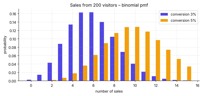
Poisson distribution
Counts of events in a fixed time or space when events happen independently at an average rate λ. Mean = variance = λ.
from scipy import stats
lam = 12                                   # calls per hour
X = stats.poisson(lam)
print("P(exactly 12 calls) =", round(X.pmf(12), 3))
print("P(more than 18)     =", round(1 - X.cdf(18), 3))
for agents_capacity in [14, 16, 18, 20]:
print(f"capacity {agents_capacity} calls/h → handles all calls {X.cdf(agents_capacity) * 100:.1f}% of hours")If each agent handles 4 calls an hour, capacity 20 needs 5 agents and covers almost every hour. Capacity 16 (4 agents) fails in roughly 1 hour out of 10. Poisson turns a guess into a service level.
Normal distribution
import numpy as np
import matplotlib.pyplot as plt
from scipy import stats
mu, sd = 30, 5                            # delivery time in minutes
x = np.linspace(10, 50, 400)
y = stats.norm.pdf(x, mu, sd)
fig, ax = plt.subplots(figsize=(9, 3.8))
ax.plot(x, y, color="#111827")
for k, c in [(3, "#e0e7ff"), (2, "#a5b4fc"), (1, "#6366f1")]:
    m = (x >= mu - k * sd) & (x <= mu + k * sd)
    ax.fill_between(x[m], y[m], color=c, label=f"±{k} SD = {stats.norm.cdf(k) - stats.norm.cdf(-k):.1%}")
ax.set_title("Delivery time ~ Normal(30, 5): the 68-95-99.7 rule"); ax.set_xlabel("minutes"); ax.legend()
plt.show()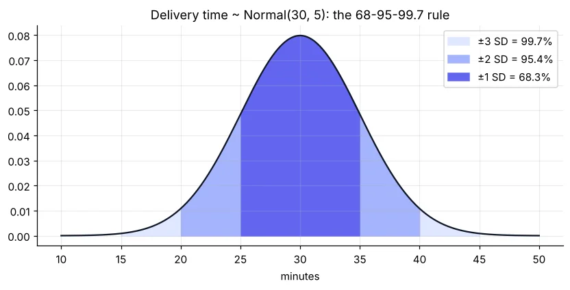
from scipy import stats
D = stats.norm(30, 5)
print("P(delivery > 40 min) =", round(1 - D.cdf(40), 4))
print("P(25 to 35 min)      =", round(D.cdf(35) - D.cdf(25), 4))
print("Promise time covering 95% of orders:", round(D.ppf(0.95), 1), "min")
print("Promise time covering 99% of orders:", round(D.ppf(0.99), 1), "min")| Method | Question it answers |
|---|---|
| pmf(k) / pdf(x) | How likely is exactly k? / density at x |
| cdf(x) | P(X ≤ x) |
| sf(x) = 1 − cdf(x) | P(X > x) |
| ppf(q) | Which value has q of the data below it? (inverse cdf) |
| rvs(size) | Generate random samples |
Is my data normal?
import pandas as pd
import matplotlib.pyplot as plt
from scipy import stats
st = pd.read_csv("students_performance.csv")
s = pd.read_csv("sales_data.csv")
fig, ax = plt.subplots(1, 2, figsize=(10, 3.8))
stats.probplot(st["average"], dist="norm", plot=ax[0]); ax[0].set_title("Student averages – close to normal")
stats.probplot(s["unit_price"], dist="norm", plot=ax[1]); ax[1].set_title("Unit prices – strongly skewed")
plt.tight_layout(); plt.show()
print("Shapiro p (students, n=500):", round(stats.shapiro(st["average"]).pvalue, 3))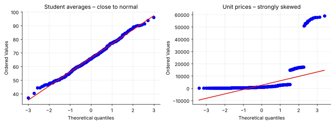
Many tests (t-test) and models (linear regression residuals) assume normality. Skewed data like prices is often log-transformed: np.log(price) is usually much closer to normal.
Real example: delivery promise from real-like data
import numpy as np
from scipy import stats
rng = np.random.default_rng(3)
times = np.round(rng.normal(32, 6, 1000), 1)          # last month's delivery times
mu, sd = times.mean(), times.std(ddof=1)
promise = stats.norm(mu, sd).ppf(0.9)
print(f"Fitted Normal: mean={mu:.1f} sd={sd:.1f}")
print(f"Promise “in {np.ceil(promise):.0f} minutes” → on time for {np.mean(times <= np.ceil(promise)) * 100:.1f}% of orders (actual)")🏅 Job skills unlocked today
Practice tasks
🏋️ Practice – do it yourself
Show solution
from scipy import stats
print(round(stats.poisson(4).sf(7), 4))
Show solution
from scipy import stats
print(round(stats.binom(10, 0.25).sf(4), 4))
Show solution
from scipy import stats
H = stats.norm(170, 7)
print(round(H.ppf(0.95), 1), "cm |", round(H.sf(185) * 100, 2), "%")
Quick quiz
🧠 Quick Quiz – test yourself
Interview corner
💼 Interview Corner
When is the normal distribution a bad assumption?
For skewed or bounded data – incomes, prices, waiting times, counts near zero, or data with heavy tails (returns, insurance claims). Check with a histogram/Q-Q plot and consider log transforms or other distributions.
Binomial vs Poisson?
Binomial counts successes in a fixed number of trials n with probability p. Poisson counts events in an interval with no fixed n. For large n and small p, Binomial(n, p) ≈ Poisson(n·p).
Summary
- Binomial: successes in n tries. Poisson: events per interval. Normal: measurements around a mean.
- cdf for “at most”, sf for “more than”, ppf for thresholds.
- 68-95-99.7 gives quick normal estimates.
- Check normality before using tests that assume it.
Day 29: sampling, the Central Limit Theorem and confidence intervals – how a survey of 1,000 can describe a city.