Day 48: NLP: Text Cleaning & Sentiment Model
✅ Today you will learn
- How computers “read” text
- Clean, tokenise and remove stop words
- Bag of words, TF-IDF and n-grams
- Train a sentiment classifier in a pipeline
- Explain predictions and know the limits
🏢 In the real world
BazaarKart receives thousands of reviews a day. The quality team cannot read them all. A sentiment model flags negative reviews within seconds and routes them to support – and the top negative words tell product teams exactly what to fix.
From words to numbers
import re
import pandas as pd
r = pd.read_csv("product_reviews.csv")
print(r["sentiment"].value_counts().to_dict())
def clean(t):
    t = t.lower()
    t = re.sub(r"[^a-z\s]", " ", t)          # keep letters only
    return re.sub(r"\s+", " ", t).strip()
r["clean"] = r["review"].apply(clean)
print(r[["review", "clean"]].head(4).to_string(index=False))Bag of words
from sklearn.feature_extraction.text import CountVectorizer
docs = ["battery life is amazing", "battery died fast, very bad", "amazing sound, amazing price"]
cv = CountVectorizer()
M = cv.fit_transform(docs)
import pandas as pd
print(pd.DataFrame(M.toarray(), columns=cv.get_feature_names_out(), index=["r1", "r2", "r3"]))
Bag of words only counts words – “not good” and “good, not bad” look similar. N-grams (pairs of words) bring back some order: ngram_range=(1, 2).
TF-IDF: important words count more
TF = how often a word appears in this review. IDF = how rare it is across all reviews. Words like “the” and “is” appear everywhere and get low weight; “refund” or “cracks” get high weight.
import pandas as pd
from sklearn.feature_extraction.text import TfidfVectorizer
r = pd.read_csv("product_reviews.csv")
tf = TfidfVectorizer(stop_words="english", ngram_range=(1, 2), min_df=2)
X = tf.fit_transform(r["review"])
print("matrix:", X.shape, "| sparsity:", round(1 - X.nnz / (X.shape[0] * X.shape[1]), 3))
row = pd.Series(X[0].toarray().ravel(), index=tf.get_feature_names_out())
print("review 0:", r.loc[0, "review"]); print(row[row > 0].sort_values(ascending=False).round(3))Train the sentiment classifier
import pandas as pd
from sklearn.model_selection import train_test_split, cross_val_score
from sklearn.pipeline import make_pipeline
from sklearn.feature_extraction.text import TfidfVectorizer
from sklearn.naive_bayes import MultinomialNB
from sklearn.linear_model import LogisticRegression
from sklearn.metrics import classification_report
r = pd.read_csv("product_reviews.csv")
X_tr, X_te, y_tr, y_te = train_test_split(r["review"], r["sentiment"], test_size=0.25, random_state=0, stratify=r["sentiment"])
for name, clf in [("Naive Bayes", MultinomialNB()), ("Logistic regression", LogisticRegression(max_iter=2000))]:
    pipe = make_pipeline(TfidfVectorizer(ngram_range=(1, 2), min_df=2), clf)
    print(f"{name:20s} 5-fold CV accuracy = {cross_val_score(pipe, X_tr, y_tr, cv=5).mean():.3f}")
best = make_pipeline(TfidfVectorizer(ngram_range=(1, 2), min_df=2), LogisticRegression(max_iter=2000)).fit(X_tr, y_tr)
print(classification_report(y_te, best.predict(X_te), digits=3))Our practice reviews are short and use clear words, so the task is easy and the score is perfect. Real review data with typos, mixed opinions and sarcasm usually gives 85–92%. A perfect score on real data should make you check for leakage.
Which words drive sentiment?
import pandas as pd
import matplotlib.pyplot as plt
from sklearn.pipeline import make_pipeline
from sklearn.feature_extraction.text import TfidfVectorizer
from sklearn.linear_model import LogisticRegression
r = pd.read_csv("product_reviews.csv")
pipe = make_pipeline(TfidfVectorizer(stop_words="english", min_df=2), LogisticRegression(max_iter=2000)).fit(r["review"], r["sentiment"])
coef = pd.Series(pipe[-1].coef_[0], index=pipe[0].get_feature_names_out())      # positive class = "positive"
top = pd.concat([coef.nsmallest(10), coef.nlargest(10)])
plt.figure(figsize=(8, 5.2))
plt.barh(top.index, top.values, color=["#dc2626" if v < 0 else "#16a34a" for v in top.values])
plt.title("Words that push a review negative (red) or positive (green)"); plt.xlabel("coefficient")
plt.show()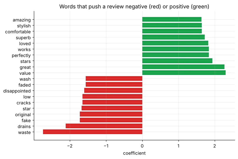
Score new reviews – and find the limits
import pandas as pd
from sklearn.pipeline import make_pipeline
from sklearn.feature_extraction.text import TfidfVectorizer
from sklearn.linear_model import LogisticRegression
r = pd.read_csv("product_reviews.csv")
pipe = make_pipeline(TfidfVectorizer(ngram_range=(1, 2), min_df=2), LogisticRegression(max_iter=2000)).fit(r["review"], r["sentiment"])
tests = ["Battery life is amazing, loved it", "Stopped working in a week, waste of money",
         "Not bad at all, quite good actually", "delivery late but product is superb",
         "bilkul bekaar product, paisa barbaad", "Phone is ok"]
for t, p in zip(tests, pipe.predict_proba(tests)[:, list(pipe.classes_).index("positive")]):
print(f"{p:5.2f} {'POS' if p >= 0.5 else 'NEG'} {t}")Negation (“not bad”), mixed reviews, sarcasm and Hinglish words it has never seen (“bekaar”, “barbaad”) confuse a bag-of-words model – unseen words are simply ignored. Fixes: collect labelled Hinglish reviews, add n-grams, or use multilingual transformer models (Day 51).
Real example: complaint topics
import pandas as pd
r = pd.read_csv("product_reviews.csv")
neg = r[r["sentiment"] == "negative"]["review"].str.lower()
topics = {"battery / charging": "battery|charg", "quality / broken": "broke|stopped|crack|faded|quality",
          "size / fit": "size|fit|tight|small", "fake / value": "fake|waste|money|original",
          "delivery": "deliver|late|courier"}
counts = {k: int(neg.str.contains(v).sum()) for k, v in topics.items()}
s = pd.Series(counts).sort_values(ascending=False)
for topic, n in s.items():
print(f"{topic:20s} {n:3d} reviews ({n / len(neg) * 100:.1f}% of negative)")🏅 Job skills unlocked today
Practice tasks
🏋️ Practice – do it yourself
Show solution
import pandas as pd
from sklearn.model_selection import train_test_split
from sklearn.pipeline import make_pipeline
from sklearn.feature_extraction.text import TfidfVectorizer
from sklearn.linear_model import LogisticRegression
from sklearn.metrics import confusion_matrix
r = pd.read_csv("product_reviews.csv")
a, b, c, d = train_test_split(r["review"], r["stars"], test_size=0.25, random_state=0, stratify=r["stars"])
m = make_pipeline(TfidfVectorizer(ngram_range=(1, 2)), LogisticRegression(max_iter=3000)).fit(a, c)
print(round(m.score(b, d), 3)); print(confusion_matrix(d, m.predict(b)))Show solution
import pandas as pd
from sklearn.model_selection import cross_val_score
from sklearn.pipeline import make_pipeline
from sklearn.feature_extraction.text import CountVectorizer
from sklearn.naive_bayes import MultinomialNB
r = pd.read_csv("product_reviews.csv")
print(round(cross_val_score(make_pipeline(CountVectorizer(), MultinomialNB()), r["review"], r["sentiment"], cv=5).mean(), 3))Quick quiz
🧠 Quick Quiz – test yourself
Interview corner
💼 Interview Corner
Explain TF-IDF.
Term frequency × inverse document frequency: a word’s weight rises with how often it appears in a document and falls with how many documents contain it, so distinctive words count more than common ones.
How would you handle Hindi/Hinglish reviews?
Collect labelled examples in that language, normalise spellings (bekar/bekaar), use character n-grams which are robust to spelling variants, or use multilingual models like IndicBERT or mBERT fine-tuned on the data.
Summary
- Text → clean → tokens → TF-IDF vectors → classifier.
- n-grams keep some word order; stop words are optional.
- Logistic regression coefficients show the words that drive sentiment.
- Bag-of-words cannot handle negation, sarcasm or unseen Hinglish well.
Day 49: time-series forecasting – trend, seasonality and predicting next month’s Delhi AQI.