Day 27: Probability for Data Science
✅ Today you will learn
- Probability as long-run frequency
- AND, OR and NOT rules
- Conditional probability from a crosstab
- Bayes’ theorem: tests, spam, fraud
- Expected value for business decisions
🏢 In the real world
A fraud system flags a UPI payment. It catches 99% of fraud and wrongly flags only 2% of normal payments. Is this payment probably fraud? Most people say “99% yes”. The real answer is closer to 5% – and Bayes’ theorem shows why. Probability thinking stops expensive mistakes.
Probability = long-run frequency
import numpy as np
rng = np.random.default_rng(42)
for n in [10, 100, 10_000, 1_000_000]:
    rolls = rng.integers(1, 7, n)
print(f"{n:>9,} dice rolls → P(six) ≈ {(rolls == 6).mean():.4f} (true = {1/6:.4f})")import numpy as np
import matplotlib.pyplot as plt
rng = np.random.default_rng(7)
flips = rng.integers(0, 2, 3000)
running = flips.cumsum() / np.arange(1, 3001)
plt.figure(figsize=(9, 3.4))
plt.plot(running, color="#4f46e5"); plt.axhline(0.5, color="#dc2626", ls="--")
plt.xscale("log"); plt.ylim(0, 1)
plt.title("Law of large numbers: share of heads settles at 0.5"); plt.xlabel("number of flips (log scale)")
plt.show()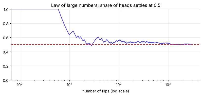
The three rules
| Rule | Formula | Example |
|---|---|---|
| NOT | P(not A) = 1 − P(A) | P(not churn) = 1 − 0.29 = 0.71 |
| OR | P(A or B) = P(A) + P(B) − P(A and B) | Senior OR monthly contract |
| AND (independent) | P(A and B) = P(A) × P(B) | Two separate customers both churn |
| AND (general) | P(A and B) = P(A) × P(B | A) | Monthly AND churn |
import pandas as pd
t = pd.read_csv("telecom_churn.csv")
A = t["senior_citizen"] == 1
B = t["contract"] == "Monthly"
pA, pB, pAB = A.mean(), B.mean(), (A & B).mean()
print(f"P(senior)={pA:.3f}  P(monthly)={pB:.3f}  P(both)={pAB:.3f}")
print(f"P(senior or monthly) by rule = {pA + pB - pAB:.3f} | counted directly = {(A | B).mean():.3f}")
print(f"P(not churn) = {1 - (t['churn'] == 'Yes').mean():.3f}")Conditional probability
P(A | B) = “probability of A given B” = P(A and B) ÷ P(B). In data, it is simply the rate inside a filtered group.
import pandas as pd
t = pd.read_csv("telecom_churn.csv")
churn = t["churn"] == "Yes"
print(f"P(churn)               = {churn.mean():.3f}")
print(f"P(churn | Monthly)     = {churn[t['contract'] == 'Monthly'].mean():.3f}")
print(f"P(churn | Two year)    = {churn[t['contract'] == 'Two year'].mean():.3f}")
print(f"P(Monthly | churn)     = {(t.loc[churn, 'contract'] == 'Monthly').mean():.3f}   ← not the same thing!")
print(pd.crosstab(t["contract"], t["churn"], margins=True))“Most churners are on monthly plans” (P(monthly | churn) ≈ 0.83) is different from “most monthly customers churn” (P(churn | monthly) ≈ 0.44). Mixing them up is one of the most common errors in reports and the news.
import pandas as pd
t = pd.read_csv("telecom_churn.csv")
churn = (t["churn"] == "Yes")
both = churn[(t["contract"] == "Monthly") & (t["tech_support"] == "No")].mean()
print(f"P(churn | monthly AND no tech support) = {both:.3f}")
print(f"Lift over average = {both / churn.mean():.2f}x")Independence
import pandas as pd
t = pd.read_csv("telecom_churn.csv")
churn = t["churn"] == "Yes"
for col in ["gender", "contract"]:
    rates = churn.groupby(t[col]).mean().round(3).to_dict()
    print(col, rates)
print("Gender: rates ≈ equal → churn looks independent of gender. Contract: very different → dependent.")Bayes' theorem
P(A | B) = P(B | A) × P(A) ÷ P(B). It updates a prior belief with new evidence.
p_fraud = 0.001          # 1 in 1,000 payments is fraud (prior)
sens = 0.99              # P(flag | fraud)
fpr = 0.02               # P(flag | normal)
p_flag = sens * p_fraud + fpr * (1 - p_fraud)
post = sens * p_fraud / p_flag
print(f"P(flag) = {p_flag:.4f}")
print(f"P(fraud | flag) = {post:.3f} → only {post * 100:.1f}% of flagged payments are fraud")import numpy as np
rng = np.random.default_rng(1)
n = 1_000_000
fraud = rng.random(n) < 0.001
flag = np.where(fraud, rng.random(n) < 0.99, rng.random(n) < 0.02)
print("Flagged payments:", flag.sum(), "| real fraud among them:", (flag & fraud).sum())
print(f"Simulated P(fraud | flag) = {(flag & fraud).sum() / flag.sum():.3f}")Do not auto-block flagged payments – that would annoy ~20,000 honest customers. Use the flag to trigger an OTP check instead. Same model, much better decision.
Expected value
# Should we give a ₹200 retention coupon to a customer with 40% churn risk?
p_churn = 0.40
monthly_bill, months_left = 700, 12
coupon = 200
p_churn_with_coupon = 0.28             # assumed from a past test
ev_no = (1 - p_churn) * monthly_bill * months_left
ev_yes = (1 - p_churn_with_coupon) * monthly_bill * months_left - coupon
print(f"Expected revenue without coupon: ₹{ev_no:,.0f}")
print(f"Expected revenue with coupon: ₹{ev_yes:,.0f} → {'give' if ev_yes > ev_no else 'skip'} the coupon")🏅 Job skills unlocked today
Practice tasks
🏋️ Practice – do it yourself
Show solution
import pandas as pd
l = pd.read_csv("loan_applications.csv")
print(round(l.loc[l["credit_score"] > 750, "approved"].mean(), 3), round(l.loc[l["credit_score"] < 650, "approved"].mean(), 3))Show solution
import numpy as np
rng = np.random.default_rng(0)
days = rng.integers(0, 365, (100_000, 30))
share = np.array([len(set(r)) < 30 for r in days])
print(round(share.mean(), 3))
Show solution
p, sens, spec = 0.02, 0.95, 0.97
print(round(sens * p / (sens * p + (1 - spec) * (1 - p)), 3))
Quick quiz
🧠 Quick Quiz – test yourself
Interview corner
💼 Interview Corner
Explain Bayes’ theorem with an example.
It updates the probability of a hypothesis using evidence: posterior = likelihood × prior ÷ evidence. Example: a fraud flag with 99% recall and 2% false-positive rate on a 0.1% base rate gives only ~5% chance a flagged payment is fraud.
What is the difference between P(A|B) and P(B|A)?
P(A|B) is the rate of A inside group B; P(B|A) is the rate of B inside group A. They are linked by Bayes’ theorem and are usually very different.
Summary
- Probability = long-run frequency; simulate to check.
- NOT, OR (subtract overlap), AND (multiply, conditional if dependent).
- P(A|B) = rate of A in group B; never confuse with P(B|A).
- Bayes: base rates matter. Expected value guides decisions.
Day 28: probability distributions – normal, binomial and Poisson, and what they predict.