Day 51: Deep Learning & Neural Networks
✅ Today you will learn
- A neuron = weighted sum + activation
- Layers, forward pass and loss
- Gradient descent and backpropagation (in NumPy)
- Train an MLP on digits with scikit-learn
- CNNs, RNNs, transformers and when deep learning is worth it
🏢 In the real world
UPI apps read cheque digits, Google Lens translates signboards, and chatbots answer in Hindi – all powered by deep learning. You do not need a GPU to understand how it works. Today you build a tiny neural network by hand, then train a real one on a laptop in seconds.
A single neuron
import numpy as np
x = np.array([0.8, 0.2, 0.5])          # study hours, absences, practice tests (scaled)
w = np.array([1.5, -2.0, 0.9])
b = -0.3
z = w @ x + b
sigmoid = lambda z: 1 / (1 + np.exp(-z))
relu = lambda z: np.maximum(0, z)
print(f"z = {z:.2f} | sigmoid → {sigmoid(z):.3f} | relu → {relu(z):.2f} | tanh → {np.tanh(z):.3f}")import numpy as np
import matplotlib.pyplot as plt
z = np.linspace(-5, 5, 200)
fig, ax = plt.subplots(1, 3, figsize=(11, 3))
for a, (name, y, c) in zip(ax, [("sigmoid", 1 / (1 + np.exp(-z)), "#4f46e5"), ("tanh", np.tanh(z), "#0891b2"), ("ReLU", np.maximum(0, z), "#dc2626")]):
a.plot(z, y, color=c, lw=2.5); a.axhline(0, color="k", lw=0.5); a.axvline(0, color="k", lw=0.5); a.set_title(name)
plt.suptitle("Activation functions add the non-linearity"); plt.tight_layout(); plt.show()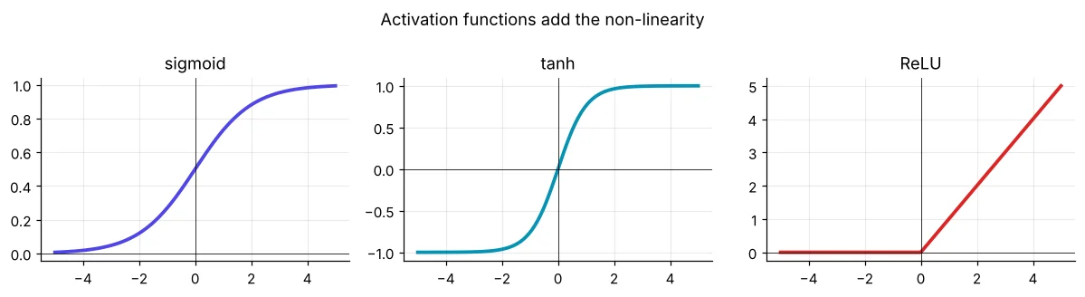
A neural network from scratch
Problem: XOR – the output is 1 when exactly one input is 1. No straight line can separate it, so logistic regression fails. One hidden layer solves it.
import numpy as np
rng = np.random.default_rng(1)
X = np.array([[0, 0], [0, 1], [1, 0], [1, 1]], dtype=float)
y = np.array([[0], [1], [1], [0]], dtype=float)
W1, b1 = rng.normal(0, 1, (2, 4)), np.zeros((1, 4))      # 2 inputs → 4 hidden neurons
W2, b2 = rng.normal(0, 1, (4, 1)), np.zeros((1, 1))      # 4 hidden → 1 output
sig = lambda z: 1 / (1 + np.exp(-z))
lr = 1.0
for epoch in range(5001):
    h = np.tanh(X @ W1 + b1)                  # forward pass
    out = sig(h @ W2 + b2)
    loss = np.mean((out - y) ** 2)
    d_out = 2 * (out - y) / len(X) * out * (1 - out)           # backpropagation
    d_h = d_out @ W2.T * (1 - h ** 2)
    W2 -= lr * h.T @ d_out; b2 -= lr * d_out.sum(0, keepdims=True)   # gradient descent step
    W1 -= lr * X.T @ d_h;   b1 -= lr * d_h.sum(0, keepdims=True)
    if epoch in (0, 500, 1000, 5000):
print(f"epoch {epoch:4d} loss {loss:.4f} predictions {out.ravel().round(2)}")- 1Forward: compute predictions layer by layer
- 2Loss: measure how wrong they are
- 3Backward: chain rule gives each weight’s blame
- 4Update: weight −= learning_rate × gradient
- 5Repeat for many epochs
A real network: handwritten digits
import time
from sklearn.datasets import load_digits
from sklearn.model_selection import train_test_split
from sklearn.preprocessing import StandardScaler
from sklearn.pipeline import make_pipeline
from sklearn.neural_network import MLPClassifier
from sklearn.linear_model import LogisticRegression
X, y = load_digits(return_X_y=True)
X_tr, X_te, y_tr, y_te = train_test_split(X, y, test_size=0.25, random_state=0, stratify=y)
for name, clf in [("logistic regression", LogisticRegression(max_iter=3000)),
                  ("MLP 64-32", MLPClassifier(hidden_layer_sizes=(64, 32), max_iter=600, random_state=0))]:
    t = time.time(); m = make_pipeline(StandardScaler(), clf).fit(X_tr, y_tr)
print(f"{name:20s} test accuracy {m.score(X_te, y_te):.3f}")import matplotlib.pyplot as plt
from sklearn.datasets import load_digits
from sklearn.model_selection import train_test_split
from sklearn.preprocessing import StandardScaler
from sklearn.neural_network import MLPClassifier
X, y = load_digits(return_X_y=True)
X_tr, X_te, y_tr, y_te = train_test_split(X, y, test_size=0.25, random_state=0, stratify=y)
sc = StandardScaler().fit(X_tr)
mlp = MLPClassifier(hidden_layer_sizes=(64, 32), max_iter=600, early_stopping=True, random_state=0).fit(sc.transform(X_tr), y_tr)
fig, ax = plt.subplots(1, 2, figsize=(11, 3.6))
ax[0].plot(mlp.loss_curve_, color="#4f46e5", label="training loss")
ax2 = ax[0].twinx(); ax2.plot(mlp.validation_scores_, color="#16a34a", label="validation accuracy")
ax[0].set_xlabel("epoch"); ax[0].set_title("Loss falls, validation accuracy rises"); ax[0].legend(loc="center right"); ax2.legend(loc="lower right")
pred = mlp.predict(sc.transform(X_te)); wrong = (pred != y_te).nonzero()[0][:6]
for i, k in enumerate(wrong):
sub = fig.add_axes([0.55 + i * 0.07, 0.25, 0.065, 0.5]); sub.imshow(X_te[k].reshape(8, 8), cmap="gray_r"); sub.axis("off")
sub.set_title(f"{y_te[k]}→{pred[k]}", fontsize=9, color="#dc2626")
ax[1].axis("off"); ax[1].set_title("Mistakes (true → predicted)")
plt.show()
print(f"stopped after {mlp.n_iter_} epochs | test accuracy {mlp.score(sc.transform(X_te), y_te):.3f}")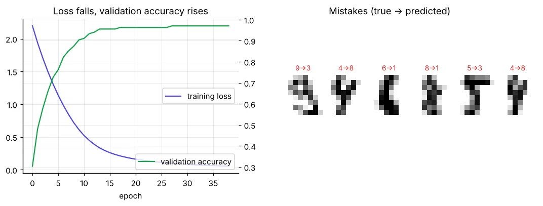
| Setting | What it controls |
|---|---|
| hidden_layer_sizes | Network shape, e.g. (64, 32) = two hidden layers |
| activation | "relu" (default), "tanh", "logistic" |
| learning_rate_init | Step size of gradient descent |
| alpha | L2 regularisation against overfitting |
| early_stopping | Stop when validation stops improving |
| batch_size | Rows per weight update |
Neural nets on business tables
import pandas as pd
from sklearn.model_selection import cross_val_score
from sklearn.preprocessing import StandardScaler
from sklearn.pipeline import make_pipeline
from sklearn.neural_network import MLPClassifier
from sklearn.ensemble import HistGradientBoostingClassifier
from sklearn.linear_model import LogisticRegression
l = pd.read_csv("loan_applications.csv"); l["lti"] = l["loan_amount"] / (l["monthly_income"] * 12)
X, y = l[["monthly_income", "credit_score", "loan_amount", "years_employed", "lti"]], l["approved"]
for name, m in [("logistic", make_pipeline(StandardScaler(), LogisticRegression())),
                ("boosting", HistGradientBoostingClassifier(learning_rate=0.05, max_iter=200, random_state=0)),
                ("MLP 32-16", make_pipeline(StandardScaler(), MLPClassifier(hidden_layer_sizes=(32, 16), alpha=1e-2, max_iter=2000, random_state=0)))]:
print(f"{name:10s} CV AUC {cross_val_score(m, X, y, cv=5, scoring='roc_auc').mean():.3f}")On small tables, simple models and boosting are as good or better – and easier to explain. Deep learning wins on images, audio, text and very large datasets where it can learn features by itself.
The deep-learning family
# pip install tensorflow   (needs more disk space; works on Google Colab out of the box)
import tensorflow as tf
from sklearn.datasets import load_digits
from sklearn.model_selection import train_test_split
X, y = load_digits(return_X_y=True)
X = X / 16.0
X_tr, X_te, y_tr, y_te = train_test_split(X, y, test_size=0.25, random_state=0, stratify=y)
model = tf.keras.Sequential([
    tf.keras.layers.Input(shape=(64,)),
    tf.keras.layers.Dense(64, activation="relu"),
    tf.keras.layers.Dropout(0.2),
    tf.keras.layers.Dense(32, activation="relu"),
    tf.keras.layers.Dense(10, activation="softmax"),
])
model.compile(optimizer="adam", loss="sparse_categorical_crossentropy", metrics=["accuracy"])
model.fit(X_tr, y_tr, epochs=30, batch_size=32, validation_split=0.1, verbose=0)
print(model.evaluate(X_te, y_te, verbose=0))
🏅 Job skills unlocked today
Practice tasks
🏋️ Practice – do it yourself
Show solution
import pandas as pd
from sklearn.model_selection import cross_val_score
from sklearn.pipeline import make_pipeline
from sklearn.compose import make_column_transformer
from sklearn.preprocessing import StandardScaler, OneHotEncoder
from sklearn.neural_network import MLPRegressor
from sklearn.linear_model import Ridge
h = pd.read_csv("house_prices.csv"); num = ["area_sqft", "bedrooms", "bathrooms", "age_years", "metro_km"]; cat = ["city", "furnishing", "parking"]
pre = make_column_transformer((StandardScaler(), num), (OneHotEncoder(), cat))
for name, m in [("Ridge", Ridge()), ("MLP", MLPRegressor(hidden_layer_sizes=(64, 32), max_iter=3000, random_state=0))]:
    s = -cross_val_score(make_pipeline(pre, m), h[num + cat], h["price_lakh"], cv=5, scoring="neg_mean_absolute_error")
print(name, round(s.mean(), 2))Quick quiz
🧠 Quick Quiz – test yourself
Interview corner
💼 Interview Corner
Explain backpropagation in simple words.
After a forward pass we measure the loss; backpropagation uses the chain rule to work backwards and find how much each weight contributed to the error, then gradient descent nudges every weight in the direction that reduces the loss.
How do you prevent overfitting in neural networks?
More data or augmentation, L2 regularisation (alpha / weight decay), dropout, early stopping on a validation set, smaller networks, and transfer learning from pre-trained models.
Summary
- Neuron = weighted sum + activation; layers stack neurons.
- Training = forward pass → loss → backprop → gradient step, repeated.
- MLPClassifier/MLPRegressor give you neural nets in scikit-learn.
- Deep learning shines on images, audio and text; boosting often wins on small tables.
Day 52: Excel and Power BI for analysts – the tools every business team already uses.