Day 43: Random Forest & Gradient Boosting
✅ Today you will learn
- Wisdom of the crowd: why ensembles win
- Random forest = bagging + random features
- Gradient boosting = trees that fix mistakes
- Key hyper-parameters and early stopping
- Permutation importance and model choice
🏢 In the real world
On real business tables – loans, churn, prices, demand – the winning models in industry and on Kaggle are almost always tree ensembles: random forests, XGBoost, LightGBM. Today you learn why, and how to use scikit-learn’s versions that need no extra installation.
Why many models beat one
import numpy as np
rng = np.random.default_rng(0)
true_price = 60.0
one_expert = rng.normal(true_price, 12, 10000)                      # one noisy guess
crowd = rng.normal(true_price, 12, (10000, 50)).mean(axis=1)        # average of 50 independent guesses
print(f"one model  : typical error ±{np.std(one_expert):.1f} lakh")
print(f"50 averaged: typical error ±{np.std(crowd):.1f} lakh")Bagging (Random Forest)
- Trees built independently, in parallel
- Each on a bootstrap sample + random features
- Average the votes → lower variance
- Hard to overfit, little tuning
Boosting (Gradient Boosting)
- Trees built one after another
- Each new tree fits the previous errors
- Small steps (learning rate) → lower bias
- Usually most accurate, needs tuning
Random forest
import pandas as pd
from sklearn.model_selection import train_test_split
from sklearn.tree import DecisionTreeRegressor
from sklearn.ensemble import RandomForestRegressor
from sklearn.metrics import mean_absolute_error
h = pd.read_csv("house_prices.csv")
X = pd.get_dummies(h.drop(columns="price_lakh"), drop_first=True, dtype=int); y = h["price_lakh"]
X_tr, X_te, y_tr, y_te = train_test_split(X, y, test_size=0.25, random_state=42)
tree = DecisionTreeRegressor(random_state=0).fit(X_tr, y_tr)
rf = RandomForestRegressor(n_estimators=300, oob_score=True, random_state=0, n_jobs=-1).fit(X_tr, y_tr)
print(f"single tree   MAE ₹{mean_absolute_error(y_te, tree.predict(X_te)):.2f} lakh")
print(f"random forest MAE ₹{mean_absolute_error(y_te, rf.predict(X_te)):.2f} lakh | OOB R² {rf.oob_score_:.3f}")Each tree sees only ~63% of rows. The rows it did not see act as a free validation set – the OOB score – so you can estimate performance without a separate split.
import pandas as pd
import matplotlib.pyplot as plt
from sklearn.model_selection import train_test_split
from sklearn.ensemble import RandomForestRegressor
from sklearn.metrics import mean_absolute_error
h = pd.read_csv("house_prices.csv")
X = pd.get_dummies(h.drop(columns="price_lakh"), drop_first=True, dtype=int); y = h["price_lakh"]
X_tr, X_te, y_tr, y_te = train_test_split(X, y, test_size=0.25, random_state=42)
ns = [1, 3, 10, 30, 100, 300]
maes = [mean_absolute_error(y_te, RandomForestRegressor(n_estimators=n, random_state=0, n_jobs=-1).fit(X_tr, y_tr).predict(X_te)) for n in ns]
plt.figure(figsize=(8, 3.6)); plt.plot(ns, maes, marker="o", color="#16a34a"); plt.xscale("log")
plt.xlabel("number of trees"); plt.ylabel("test MAE (₹ lakh)"); plt.title("More trees → lower error, then it levels off")
plt.show()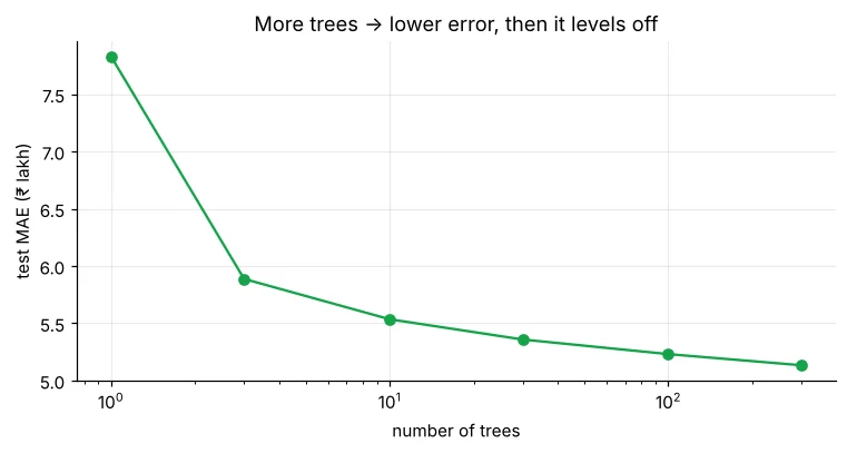
Gradient boosting
import numpy as np
import pandas as pd
from sklearn.tree import DecisionTreeRegressor
h = pd.read_csv("house_prices.csv"); p = h[h["city"] == "Pune"]
X, y = p[["area_sqft", "metro_km", "age_years"]], p["price_lakh"].to_numpy()
pred = np.full(len(y), y.mean())                       # start with the average
lr = 0.3
for step in range(1, 6):
    resid = y - pred                                   # what we still get wrong
    t = DecisionTreeRegressor(max_depth=2, random_state=0).fit(X, resid)
    pred = pred + lr * t.predict(X)                    # take a small step
print(f"step {step}: mean absolute error = {np.abs(y - pred).mean():.2f} lakh")import pandas as pd
from sklearn.model_selection import train_test_split
from sklearn.ensemble import RandomForestRegressor, HistGradientBoostingRegressor
from sklearn.linear_model import LinearRegression
from sklearn.metrics import mean_absolute_error
h = pd.read_csv("house_prices.csv")
X = pd.get_dummies(h.drop(columns="price_lakh"), drop_first=True, dtype=int); y = h["price_lakh"]
X_tr, X_te, y_tr, y_te = train_test_split(X, y, test_size=0.25, random_state=42)
models = {"Linear regression": LinearRegression(),
"Random forest": RandomForestRegressor(n_estimators=300, random_state=0, n_jobs=-1),
"Hist gradient boosting": HistGradientBoostingRegressor(learning_rate=0.05, max_iter=600, early_stopping=True, random_state=0)}
for name, m in models.items():
m.fit(X_tr, y_tr)
print(f"{name:24s} MAE ₹{mean_absolute_error(y_te, m.predict(X_te)):.2f} lakh")
print("boosting stopped after", models["Hist gradient boosting"].n_iter_, "trees (early stopping)")House prices in our data follow a mostly multiplicative formula (area × city rate × small % effects). A linear model on good features captures that well. Ensembles shine when relationships are messy and interacting – like churn and loans below. Always compare!
Classification: the loan model
import pandas as pd
from sklearn.model_selection import train_test_split
from sklearn.linear_model import LogisticRegression
from sklearn.tree import DecisionTreeClassifier
from sklearn.ensemble import RandomForestClassifier, HistGradientBoostingClassifier
from sklearn.metrics import roc_auc_score, accuracy_score
l = pd.read_csv("loan_applications.csv")
l["lti"] = l["loan_amount"] / (l["monthly_income"] * 12); l["salaried"] = (l["employment"] == "Salaried").astype(int)
X = l[["monthly_income", "credit_score", "loan_amount", "years_employed", "salaried"]]   # no lti – let models find it
y = l["approved"]
X_tr, X_te, y_tr, y_te = train_test_split(X, y, test_size=0.25, random_state=42, stratify=y)
models = {"Logistic": LogisticRegression(max_iter=5000), "Tree": DecisionTreeClassifier(max_depth=5, random_state=0),
          "Random forest": RandomForestClassifier(n_estimators=400, min_samples_leaf=3, random_state=0, n_jobs=-1),
          "Gradient boosting": HistGradientBoostingClassifier(learning_rate=0.05, max_iter=300, random_state=0)}
for name, m in models.items():
    p = m.fit(X_tr, y_tr).predict_proba(X_te)[:, 1]
print(f"{name:18s} accuracy={accuracy_score(y_te, p > 0.5):.3f} AUC={roc_auc_score(y_te, p):.3f}")Without the hand-made loan_to_income feature, the linear model struggles, while forests and boosting discover the income × loan interaction on their own. With good features, simple models catch up – feature engineering still matters.
Hyper-parameters that matter
| Model | Parameter | Typical values | Effect |
|---|---|---|---|
| Random forest | n_estimators | 200–1000 | More = stabler, slower |
| Random forest | max_features | "sqrt", 0.3–0.6 | Randomness between trees |
| Random forest | min_samples_leaf | 1–20 | Bigger = smoother |
| Boosting | learning_rate | 0.01–0.2 | Smaller = needs more trees, often better |
| Boosting | max_iter + early_stopping | 200–2000 | Stops when validation stops improving |
| Boosting | max_depth / max_leaf_nodes | 3–8 / 15–63 | Tree complexity |
Which features drive the model?
import pandas as pd
import matplotlib.pyplot as plt
from sklearn.model_selection import train_test_split
from sklearn.ensemble import RandomForestClassifier
from sklearn.inspection import permutation_importance
l = pd.read_csv("loan_applications.csv"); l["salaried"] = (l["employment"] == "Salaried").astype(int)
X = l[["monthly_income", "credit_score", "loan_amount", "years_employed", "salaried"]]; y = l["approved"]
X_tr, X_te, y_tr, y_te = train_test_split(X, y, test_size=0.25, random_state=42, stratify=y)
rf = RandomForestClassifier(n_estimators=400, min_samples_leaf=3, random_state=0, n_jobs=-1).fit(X_tr, y_tr)
pi = permutation_importance(rf, X_te, y_te, n_repeats=20, random_state=0, scoring="roc_auc")
imp = pd.Series(pi.importances_mean, index=X.columns).sort_values()
imp.plot(kind="barh", figsize=(7.5, 3.4), color="#4f46e5")
plt.title("Permutation importance: AUC drop when a feature is shuffled"); plt.xlabel("AUC drop"); plt.show()
print(imp.round(3).sort_values(ascending=False).to_string())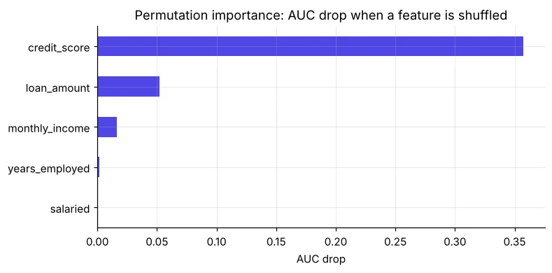
feature_importances_ of trees favours features with many unique values (like income). Permutation importance on the test set is more reliable.
Which model should I use?
🏅 Job skills unlocked today
Practice tasks
🏋️ Practice – do it yourself
Show solution
import pandas as pd
from sklearn.model_selection import train_test_split
from sklearn.ensemble import RandomForestRegressor
from sklearn.linear_model import LinearRegression
st = pd.read_csv("students_performance.csv")
X = pd.get_dummies(st.drop(columns=["student_id", "maths", "science", "english", "average", "result"]), drop_first=True, dtype=int)
a, b, c, d = train_test_split(X, st["average"], test_size=0.25, random_state=0)
for m in [LinearRegression(), RandomForestRegressor(n_estimators=300, random_state=0)]:
print(type(m).__name__, round(m.fit(a, c).score(b, d), 3))Show solution
import pandas as pd
from sklearn.model_selection import train_test_split
from sklearn.ensemble import HistGradientBoostingClassifier
from sklearn.metrics import roc_auc_score
l = pd.read_csv("loan_applications.csv")
X, y = l[["monthly_income", "credit_score", "loan_amount", "years_employed"]], l["approved"]
a, b, c, d = train_test_split(X, y, test_size=0.25, random_state=42, stratify=y)
for lr in [0.3, 0.1, 0.03]:
    m = HistGradientBoostingClassifier(learning_rate=lr, max_iter=1000, early_stopping=True, random_state=0).fit(a, c)
print(lr, round(roc_auc_score(d, m.predict_proba(b)[:, 1]), 3), m.n_iter_)lti feature to the loan comparison. How much does logistic regression improve?Quick quiz
🧠 Quick Quiz – test yourself
Interview corner
💼 Interview Corner
Explain the difference between bagging and boosting.
Bagging trains many models independently on bootstrap samples and averages them, reducing variance (random forest). Boosting trains models sequentially, each correcting the previous errors, reducing bias (gradient boosting, XGBoost).
Why might a random forest overfit less than a single tree?
Each tree sees a different bootstrap sample and random subset of features, so their errors are less correlated; averaging cancels much of the noise each tree memorised.
Summary
- Ensembles combine many trees: bagging lowers variance, boosting lowers bias.
- Random forest: robust default, OOB score, little tuning.
- Gradient boosting: learning rate + early stopping, top accuracy.
- Compare with linear baselines and use permutation importance.
Day 44: feature engineering and scaling – encoding, scaling, binning, interactions and avoiding leakage.