Day 30: Hypothesis Testing: t-test & Chi-square
✅ Today you will learn
- H₀, H₁, α and the 5-step process
- p-value – what it is and is not
- t-tests: one-sample, two-sample, paired
- Chi-square for categories, ANOVA for 3+ groups
- Type I/II errors, effect size, which test when
🏢 In the real world
Customers with tech support churn 25%, those without 37%. A manager says “obviously tech support works – give it to everyone!” A sceptic says “it is just random noise”. A hypothesis test settles the argument with evidence, not opinions.
The 5-step process
- 1State H₀ (no effect) and H₁ (effect)
- 2Choose α (usually 0.05)
- 3Pick the test and compute the statistic
- 4Get the p-value
- 5Decide and explain in business words
H₀ = “innocent” (no difference). We need strong evidence (small p-value) to reject it. Not rejecting H₀ does not prove innocence – it means not enough evidence.
The p-value by simulation
p-value = if H₀ were true, how often would we see a difference at least this big just by chance?
import numpy as np
import pandas as pd
t = pd.read_csv("telecom_churn.csv")
t = t[t["tech_support"] != "No internet"]
churn = (t["churn"] == "Yes").to_numpy()
has_ts = (t["tech_support"] == "Yes").to_numpy()
observed = churn[~has_ts].mean() - churn[has_ts].mean()
rng = np.random.default_rng(0)
diffs = []
for _ in range(5000):                       # shuffle labels = world where H0 is true
    lab = rng.permutation(has_ts)
    diffs.append(churn[~lab].mean() - churn[lab].mean())
diffs = np.array(diffs)
print(f"Observed difference: {observed:.3f}")
print(f"Largest shuffled difference: {diffs.max():.3f}")
print(f"p-value ≈ {(np.abs(diffs) >= abs(observed)).mean():.4f}")import numpy as np
import pandas as pd
import matplotlib.pyplot as plt
t = pd.read_csv("telecom_churn.csv"); t = t[t["tech_support"] != "No internet"]
churn = (t["churn"] == "Yes").to_numpy(); ts = (t["tech_support"] == "Yes").to_numpy()
obs = churn[~ts].mean() - churn[ts].mean()
rng = np.random.default_rng(0)
d = [churn[~(l := rng.permutation(ts))].mean() - churn[l].mean() for _ in range(5000)]
plt.figure(figsize=(9, 3.5))
plt.hist(d, bins=40, color="#cbd5e1", label="differences if H₀ were true")
plt.axvline(obs, color="#dc2626", lw=2.5, label=f"observed = {obs:.3f}")
plt.title("The real difference is far outside what chance produces → reject H₀"); plt.legend()
plt.show()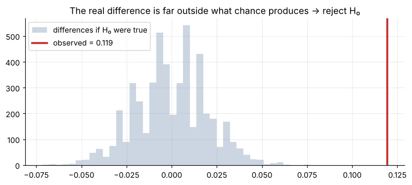
| p-value | Plain meaning |
|---|---|
| < 0.01 | Very strong evidence against H₀ |
| 0.01–0.05 | Evidence against H₀ (significant at 5%) |
| 0.05–0.10 | Weak evidence – collect more data |
| > 0.10 | No evidence of a difference |
It is not the probability that H₀ is true, and it says nothing about how big or important the effect is. With huge data, tiny useless differences become “significant”. Always report the effect size too.
t-tests
import pandas as pd
from scipy import stats
s = pd.read_csv("sales_data.csv")
r = s["rating"].dropna()
# One-sample: is the average rating different from the target 4.0?
res = stats.ttest_1samp(r, 4.0)
print(f"mean {r.mean():.3f} | t={res.statistic:.2f} p={res.pvalue:.4f}")import pandas as pd
from scipy import stats
t = pd.read_csv("telecom_churn.csv")
yes = t.loc[t["churn"] == "Yes", "monthly_charges"]
no = t.loc[t["churn"] == "No", "monthly_charges"]
res = stats.ttest_ind(yes, no, equal_var=False) # Welch’s t-test (safer)
pooled = ((yes.var() + no.var()) / 2) ** 0.5
print(f"churners ₹{yes.mean():.0f} vs stayers ₹{no.mean():.0f}")
print(f"t={res.statistic:.2f}, p={res.pvalue:.2e}, Cohen's d={(yes.mean() - no.mean()) / pooled:.2f}")import numpy as np
from scipy import stats
rng = np.random.default_rng(4)
before = rng.normal(62, 9, 40).round() # mock-test marks before a crash course
after = (before + rng.normal(3, 4, 40)).round() # same 40 students after
res = stats.ttest_rel(after, before)
print(f"avg gain {np.mean(after - before):.2f} marks | t={res.statistic:.2f} p={res.pvalue:.4f}")Chi-square: two categorical variables
import pandas as pd
from scipy import stats
t = pd.read_csv("telecom_churn.csv")
for col in ["contract", "gender"]:
    table = pd.crosstab(t[col], t["churn"])
    chi2, p, dof, expected = stats.chi2_contingency(table)
    print(f"{col:9s} chi2={chi2:7.1f} dof={dof} p={p:.3g}")
print(pd.crosstab(t["gender"], t["churn"]))ANOVA: three or more groups
import pandas as pd
from scipy import stats
h = pd.read_csv("house_prices.csv")
h["ppsf"] = h["price_lakh"] * 1e5 / h["area_sqft"]
groups = [g["ppsf"] for _, g in h.groupby("furnishing")]
f, p = stats.f_oneway(*groups)
print(h.groupby("furnishing")["ppsf"].mean().round(0).to_dict())
print(f"ANOVA F={f:.2f}, p={p:.4f}")Errors and power
| H₀ true | H₀ false | |
|---|---|---|
| Reject H₀ | Type I error (false alarm), rate = α | Correct (power) |
| Keep H₀ | Correct | Type II error (missed effect), rate = β |
import numpy as np
from scipy import stats
rng = np.random.default_rng(0)
false_alarms = sum(stats.ttest_ind(rng.normal(0, 1, 50), rng.normal(0, 1, 50)).pvalue < 0.05 for _ in range(2000))
print(f"No real difference, yet 'significant' in {false_alarms / 2000:.1%} of tests (≈ α)")
for n in [20, 50, 200]:
    power = np.mean([stats.ttest_ind(rng.normal(0, 1, n), rng.normal(0.3, 1, n)).pvalue < 0.05 for _ in range(2000)])
print(f"real small effect (d=0.3), n={n:3d} per group → detected {power:.0%} of the time")Which test should I use?
| Question | Data | Test (scipy.stats) |
|---|---|---|
| Mean vs a target | 1 numeric | ttest_1samp |
| Two group means | numeric + 2 groups | ttest_ind (equal_var=False) |
| Before vs after, same people | 2 paired numeric | ttest_rel |
| 3+ group means | numeric + 3+ groups | f_oneway |
| Two categories related? | 2 categorical | chi2_contingency |
| Two proportions | counts | proportions_ztest (statsmodels) – Day 31 |
| Non-normal / ranks | numeric | mannwhitneyu, kruskal |
🏅 Job skills unlocked today
Practice tasks
🏋️ Practice – do it yourself
Show solution
import pandas as pd
from scipy import stats
st = pd.read_csv("students_performance.csv")
a = st.loc[st["internet"] == "Yes", "average"]; b = st.loc[st["internet"] == "No", "average"]
print(f"difference {a.mean() - b.mean():.2f} marks, p = {stats.ttest_ind(a, b, equal_var=False).pvalue:.4f}")Show solution
import pandas as pd
from scipy import stats
s = pd.read_csv("sales_data.csv")
chi2, p, dof, _ = stats.chi2_contingency(pd.crosstab(s["region"], s["payment_mode"]))
print(round(chi2, 2), dof, round(p, 4))Show solution
import pandas as pd
from scipy import stats
h = pd.read_csv("house_prices.csv"); h["ppsf"] = h["price_lakh"] * 1e5 / h["area_sqft"]
r = stats.f_oneway(*[g["ppsf"] for _, g in h.groupby("city")])
print(f"F={r.statistic:.1f}, p={r.pvalue:.1e}")Quick quiz
🧠 Quick Quiz – test yourself
Interview corner
💼 Interview Corner
Explain a p-value to a non-technical person.
“If there were truly no difference, a gap this big would happen by chance only p×100 times in 100. Since that is very rare, we believe the difference is real.” Then add how big the difference is.
Statistically significant vs practically significant?
Statistical significance says the effect is unlikely to be noise. Practical significance asks if it is big enough to matter (₹ impact, effect size). With millions of rows, a 0.1% lift can be significant but worthless.
Summary
- H₀ = no effect; small p-value = evidence against it.
- p-value is not P(H₀ true) and not effect size.
- t-tests for means, chi-square for categories, ANOVA for 3+ groups.
- Mind Type I/II errors, power and multiple testing.
Day 31: correlation and A/B testing – run a complete website experiment from design to decision.