Day 40: Logistic Regression: Loan Approval
✅ Today you will learn
- Why linear regression fails for yes/no
- The sigmoid: score → probability
- Fit, predict_proba and coefficients
- Odds ratios in plain language
- Choose a threshold for the business
🏢 In the real world
Regulators want banks to explain every loan decision. A black-box model is risky; logistic regression gives a probability and a clear reason – “each extra 50 points of credit score multiplies your odds of approval by about 5”. That is why it is still the most used model in Indian banking and insurance.
Why not linear regression?
import numpy as np
import pandas as pd
import matplotlib.pyplot as plt
from sklearn.linear_model import LinearRegression, LogisticRegression
l = pd.read_csv("loan_applications.csv")
X, y = l[["credit_score"]], l["approved"]
lin = LinearRegression().fit(X, y); log = LogisticRegression().fit(X, y)
grid = pd.DataFrame({"credit_score": np.linspace(450, 900, 200)})
jit = y + np.random.default_rng(0).uniform(-0.04, 0.04, len(y))
plt.figure(figsize=(9, 4))
plt.scatter(l["credit_score"], jit, s=6, alpha=0.3, color="#64748b", label="applications (0 = reject, 1 = approve)")
plt.plot(grid, lin.predict(grid), color="#f59e0b", lw=2, label="linear regression (goes below 0 / above 1!)")
plt.plot(grid, log.predict_proba(grid)[:, 1], color="#4f46e5", lw=3, label="logistic regression (S-curve)")
plt.axhline(0.5, color="#dc2626", ls=":", lw=1); plt.ylim(-0.3, 1.3); plt.xlabel("credit score"); plt.legend(fontsize=8)
plt.title("Logistic regression keeps probabilities between 0 and 1"); plt.show()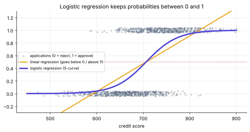
The sigmoid function
score z = b₀ + b₁x₁ + b₂x₂ + … then probability = 1 / (1 + e−z). z is the log-odds.
import numpy as np
sigmoid = lambda z: 1 / (1 + np.exp(-z))
for z in [-4, -2, 0, 2, 4]:
    p = sigmoid(z)
print(f"z={z:+d} → probability {p:.3f} → odds {p / (1 - p):6.2f}")Fit the loan model
import pandas as pd
from sklearn.model_selection import train_test_split
from sklearn.linear_model import LogisticRegression
from sklearn.preprocessing import StandardScaler
from sklearn.pipeline import make_pipeline
l = pd.read_csv("loan_applications.csv")
l["loan_to_income"] = l["loan_amount"] / (l["monthly_income"] * 12)
l["is_salaried"] = (l["employment"] == "Salaried").astype(int)
feats = ["credit_score", "loan_to_income", "years_employed", "is_salaried", "monthly_income"]
X_tr, X_te, y_tr, y_te = train_test_split(l[feats], l["approved"], test_size=0.25, random_state=42, stratify=l["approved"])
model = make_pipeline(StandardScaler(), LogisticRegression()).fit(X_tr, y_tr)
print(f"test accuracy = {model.score(X_te, y_te):.3f}")
print(pd.Series(model[-1].coef_[0], index=feats).round(3).sort_values().to_string())After StandardScaler, coefficients are “per 1 standard deviation” and comparable: the biggest absolute value is the strongest driver. Here loan-to-income (negative) and credit score (positive) dominate; monthly income adds little once loan-to-income is known.
Odds ratios – the explanation regulators like
import numpy as np
import pandas as pd
from sklearn.linear_model import LogisticRegression
l = pd.read_csv("loan_applications.csv")
l["loan_to_income"] = l["loan_amount"] / (l["monthly_income"] * 12)
l["is_salaried"] = (l["employment"] == "Salaried").astype(int)
feats = ["credit_score", "loan_to_income", "years_employed", "is_salaried"]
m = LogisticRegression(max_iter=5000).fit(l[feats], l["approved"])
c = pd.Series(m.coef_[0], index=feats)
print(f"+50 credit points  → odds × {np.exp(50 * c['credit_score']):.2f}")
print(f"+0.5 loan/income   → odds × {np.exp(0.5 * c['loan_to_income']):.2f}")
print(f"+5 years employed  → odds × {np.exp(5 * c['years_employed']):.2f}")
print(f"salaried vs not → odds × {np.exp(c['is_salaried']):.2f}")“Your application was declined mainly because the loan is 2.5× your yearly income. Reducing the loan to 1.2× your income would raise your approval chance from about 12% to about 48%.” (salaried, score 700, 5 years) Logistic regression makes such explanations easy.
Choosing the threshold
import numpy as np
import pandas as pd
from sklearn.model_selection import train_test_split
from sklearn.linear_model import LogisticRegression
l = pd.read_csv("loan_applications.csv")
l["lti"] = l["loan_amount"] / (l["monthly_income"] * 12)
X = l[["credit_score", "lti", "years_employed"]]; y = l["approved"]
X_tr, X_te, y_tr, y_te = train_test_split(X, y, test_size=0.25, random_state=42, stratify=y)
p = LogisticRegression(max_iter=5000).fit(X_tr, y_tr).predict_proba(X_te)[:, 1]
print("threshold  approved%  accuracy  wrongly_approved")
for t in [0.3, 0.5, 0.7, 0.85]:
    pred = (p >= t).astype(int)
print(f" {t:.2f} {pred.mean():6.1%} {np.mean(pred == y_te):.3f} {np.sum((pred == 1) & (y_te == 0)):3d}")A cautious bank raises the threshold to approve fewer bad loans; a growth-focused NBFC lowers it to approve more customers. The model gives probabilities – the business chooses the cut-off. Day 41 shows how to pick it with precision and recall.
The decision boundary
import numpy as np
import pandas as pd
import matplotlib.pyplot as plt
from sklearn.linear_model import LogisticRegression
l = pd.read_csv("loan_applications.csv")
l["lti"] = l["loan_amount"] / (l["monthly_income"] * 12)
X = l[["credit_score", "lti"]]; y = l["approved"]
m = LogisticRegression(max_iter=5000).fit(X, y)
xx, yy = np.meshgrid(np.linspace(480, 900, 200), np.linspace(0, 3, 200))
zz = m.predict_proba(pd.DataFrame({"credit_score": xx.ravel(), "lti": yy.ravel()}))[:, 1].reshape(xx.shape)
plt.figure(figsize=(8.5, 4.6))
cs = plt.contourf(xx, yy, zz, levels=10, cmap="RdYlGn", alpha=0.55); plt.colorbar(cs, label="P(approve)")
plt.contour(xx, yy, zz, levels=[0.5], colors="black", linewidths=2)
plt.scatter(X["credit_score"], X["lti"], c=y, cmap="RdYlGn", edgecolor="k", s=10, linewidths=0.3)
plt.xlabel("credit score"); plt.ylabel("loan ÷ yearly income"); plt.ylim(0, 3)
plt.title("Black line = 50% boundary: high score + small loan → approve"); plt.show()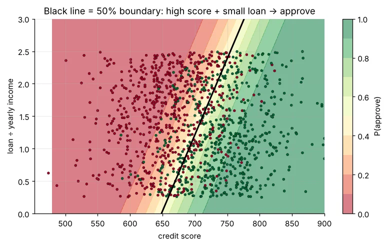
Real example: a simple scorecard
import numpy as np
import pandas as pd
from sklearn.linear_model import LogisticRegression
l = pd.read_csv("loan_applications.csv")
l["lti"] = l["loan_amount"] / (l["monthly_income"] * 12)
l["salaried"] = (l["employment"] == "Salaried").astype(int)
feats = ["credit_score", "lti", "years_employed", "salaried"]
m = LogisticRegression(max_iter=5000).fit(l[feats], l["approved"])
def explain(app):
    x = pd.DataFrame([app])[feats]
    contrib = (x.iloc[0] - l[feats].mean()) * m.coef_[0]
    p = m.predict_proba(x)[0, 1]
    print(f"P(approve) = {p:.0%}  | biggest factors:", contrib.sort_values(key=abs, ascending=False).round(2).head(2).to_dict())
explain({"credit_score": 760, "lti": 0.8, "years_employed": 8, "salaried": 1})
explain({"credit_score": 690, "lti": 2.4, "years_employed": 3, "salaried": 0})🏅 Job skills unlocked today
Practice tasks
🏋️ Practice – do it yourself
Show solution
import numpy as np, pandas as pd
from sklearn.linear_model import LogisticRegression
st = pd.read_csv("students_performance.csv")
X = st[["study_hours", "attendance"]].assign(internet=(st["internet"] == "Yes").astype(int)); y = (st["average"] >= 75).astype(int)
m = LogisticRegression(max_iter=5000).fit(X, y)
print("odds × per study hour:", round(np.exp(m.coef_[0][0]), 2))Show solution
import numpy as np, pandas as pd
from sklearn.linear_model import LogisticRegression
l = pd.read_csv("loan_applications.csv"); l["lti"] = l["loan_amount"] / (l["monthly_income"] * 12); l["sal"] = (l["employment"] == "Salaried").astype(int)
m = LogisticRegression(max_iter=5000).fit(l[["credit_score", "lti", "years_employed", "sal"]], l["approved"])
grid = pd.DataFrame({"credit_score": range(500, 901), "lti": 1.0, "years_employed": 5, "sal": 1})
p = m.predict_proba(grid)[:, 1]; print("≈", grid["credit_score"][np.argmax(p >= 0.5)])Quick quiz
🧠 Quick Quiz – test yourself
Interview corner
💼 Interview Corner
How do you interpret a logistic regression coefficient?
It is the change in log-odds for a one-unit increase in the feature, holding others fixed. exp(coef) is the odds ratio: e.g. 1.5 means the odds increase by 50% per unit.
Why is logistic regression popular in banking?
It is fast, stable, gives calibrated probabilities, and is easy to explain and audit with odds ratios and reason codes – important for regulators and customers.
Summary
- Logistic regression = linear score → sigmoid → probability.
- exp(coef) = odds ratio – easy to explain.
- Scale features to compare coefficients.
- The business chooses the threshold, not the model.
Day 41: classification metrics – confusion matrix, precision, recall, F1, ROC-AUC and choosing the right one.