दिन 39: Multiple Regression, Ridge और Lasso

import pandas as pd
h = pd.read_csv("house_prices.csv")
X = pd.get_dummies(h.drop(columns="price_lakh"), columns=["city", "furnishing", "parking"], drop_first=True, dtype=int)
print(X.columns.tolist())
print(X.head(3))

import pandas as pd
from sklearn.model_selection import train_test_split
from sklearn.linear_model import LinearRegression
from sklearn.metrics import mean_absolute_error, r2_score
h = pd.read_csv("house_prices.csv")
X = pd.get_dummies(h.drop(columns="price_lakh"), columns=["city", "furnishing", "parking"], drop_first=True, dtype=int)
y = h["price_lakh"]
X_tr, X_te, y_tr, y_te = train_test_split(X, y, test_size=0.25, random_state=42)
area_only = LinearRegression().fit(X_tr[["area_sqft"]], y_tr)
full = LinearRegression().fit(X_tr, y_tr)
for name, m, cols in [("area only", area_only, ["area_sqft"]), ("all features", full, X.columns)]:
    p = m.predict(X_te[cols])
    print(f"{name:13s} MAE = ₹{mean_absolute_error(y_te, p):.2f} lakh   R² = {r2_score(y_te, p):.3f}")

import pandas as pd
from sklearn.linear_model import LinearRegression
h = pd.read_csv("house_prices.csv")
X = pd.get_dummies(h.drop(columns="price_lakh"), columns=["city", "furnishing", "parking"], drop_first=True, dtype=int)
m = LinearRegression().fit(X, h["price_lakh"])
coef = pd.Series(m.coef_, index=X.columns).round(3)
print(coef.sort_values().to_string())

import pandas as pd
from statsmodels.stats.outliers_influence import variance_inflation_factor
h = pd.read_csv("house_prices.csv")
num = h[["area_sqft", "bedrooms", "bathrooms", "age_years", "metro_km"]].assign(const=1)
vif = pd.Series([variance_inflation_factor(num.values, i) for i in range(num.shape[1] - 1)], index=num.columns[:-1]).round(2)
print(vif.to_string())
print("VIF > 5 → strongly explained by the other features")

import numpy as np
import pandas as pd
from sklearn.model_selection import train_test_split
from sklearn.linear_model import LinearRegression
from sklearn.metrics import mean_absolute_error
h = pd.read_csv("house_prices.csv")
X = pd.get_dummies(h.drop(columns="price_lakh"), columns=["city", "furnishing", "parking"], drop_first=True, dtype=int)
X["log_area"] = np.log(X["area_sqft"])
y = h["price_lakh"]
X_tr, X_te, y_tr, y_te = train_test_split(X, y, test_size=0.25, random_state=42)
plain = LinearRegression().fit(X_tr.drop(columns="log_area"), y_tr)
logm = LinearRegression().fit(X_tr.drop(columns="area_sqft"), np.log(y_tr))
p1 = plain.predict(X_te.drop(columns="log_area"))
p2 = np.exp(logm.predict(X_te.drop(columns="area_sqft")))
print(f"price model     MAE = ₹{mean_absolute_error(y_te, p1):.2f} lakh")
print(f"log-price model MAE = ₹{mean_absolute_error(y_te, p2):.2f} lakh")
c = pd.Series(logm.coef_, index=X_tr.drop(columns="area_sqft").columns)
print(f"each km from metro → {(np.exp(c['metro_km']) - 1) * 100:.1f}% price | furnished → {(np.exp(c['furnishing_Unfurnished']) - 1) * -100:.1f}% more than unfurnished")

import numpy as np
import pandas as pd
from sklearn.model_selection import train_test_split
from sklearn.linear_model import LinearRegression, Ridge, Lasso
from sklearn.preprocessing import StandardScaler
from sklearn.pipeline import make_pipeline
h = pd.read_csv("house_prices.csv")
X = pd.get_dummies(h.drop(columns="price_lakh"), columns=["city", "furnishing", "parking"], drop_first=True, dtype=int)
rng = np.random.default_rng(0)
for i in range(30):                                   # add 30 useless noise columns
    X[f"noise_{i}"] = rng.normal(size=len(X))
X_tr, X_te, y_tr, y_te = train_test_split(X, h["price_lakh"], test_size=0.5, random_state=1)
for name, est in [("Linear", LinearRegression()), ("Ridge α=10", Ridge(alpha=10)), ("Lasso α=0.3", Lasso(alpha=0.3, max_iter=20000))]:
    m = make_pipeline(StandardScaler(), est).fit(X_tr, y_tr)
    coefs = m[-1].coef_
    print(f"{name:12s} test R²={m.score(X_te, y_te):.3f} | non-zero coefs={np.sum(np.abs(coefs) > 1e-6):2d} of {len(coefs)}")

import numpy as np
import pandas as pd
import matplotlib.pyplot as plt
from sklearn.linear_model import Lasso
from sklearn.preprocessing import StandardScaler
h = pd.read_csv("house_prices.csv")
X = pd.get_dummies(h.drop(columns="price_lakh"), columns=["city", "furnishing", "parking"], drop_first=True, dtype=int)
Xs = StandardScaler().fit_transform(X)
alphas = np.logspace(-2, 1.3, 40)
paths = np.array([Lasso(alpha=a, max_iter=20000).fit(Xs, h["price_lakh"]).coef_ for a in alphas])
plt.figure(figsize=(9, 4.2))
for j, col in enumerate(X.columns):
    plt.plot(alphas, paths[:, j], label=col if j < 9 else None)
plt.xscale("log"); plt.axhline(0, color="black", lw=0.6)
plt.xlabel("alpha (penalty strength)"); plt.ylabel("coefficient (scaled)")
plt.title("Lasso path: weak features drop to zero first; area survives longest")
plt.legend(fontsize=7, ncol=2); plt.show()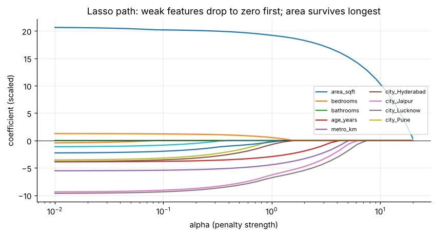

import pandas as pd
from sklearn.linear_model import RidgeCV, LassoCV
from sklearn.preprocessing import StandardScaler
from sklearn.pipeline import make_pipeline
h = pd.read_csv("house_prices.csv")
X = pd.get_dummies(h.drop(columns="price_lakh"), columns=["city", "furnishing", "parking"], drop_first=True, dtype=int)
ridge = make_pipeline(StandardScaler(), RidgeCV(alphas=[0.01, 0.1, 1, 10, 100])).fit(X, h["price_lakh"])
lasso = make_pipeline(StandardScaler(), LassoCV(cv=5, random_state=0, max_iter=20000)).fit(X, h["price_lakh"])
print("best Ridge alpha:", ridge[-1].alpha_, "| best Lasso alpha:", round(lasso[-1].alpha_, 4))