दिन 51: Deep Learning और Neural Networks
✅ आज आप सीखेंगे
- Neuron = weighted sum + activation
- Layers, forward pass और loss
- Gradient descent और backpropagation (NumPy में)
- scikit-learn से digits पर MLP train करना
- CNNs, RNNs, transformers और deep learning कब फ़ायदेमंद
🏢 असली दुनिया में
UPI apps cheque के अंक पढ़ते हैं, Google Lens signboards translate करता है, और chatbots Hindi में जवाब देते हैं – सब deep learning से। यह कैसे काम करता है, समझने के लिए GPU नहीं चाहिए। आज आप हाथ से छोटा neural network बनाएँगे, फिर laptop पर सेकंडों में असली network train करेंगे।
एक neuron
import numpy as np
x = np.array([0.8, 0.2, 0.5])          # study hours, absences, practice tests (scaled)
w = np.array([1.5, -2.0, 0.9])
b = -0.3
z = w @ x + b
sigmoid = lambda z: 1 / (1 + np.exp(-z))
relu = lambda z: np.maximum(0, z)
print(f"z = {z:.2f} | sigmoid → {sigmoid(z):.3f} | relu → {relu(z):.2f} | tanh → {np.tanh(z):.3f}")import numpy as np
import matplotlib.pyplot as plt
z = np.linspace(-5, 5, 200)
fig, ax = plt.subplots(1, 3, figsize=(11, 3))
for a, (name, y, c) in zip(ax, [("sigmoid", 1 / (1 + np.exp(-z)), "#4f46e5"), ("tanh", np.tanh(z), "#0891b2"), ("ReLU", np.maximum(0, z), "#dc2626")]):
a.plot(z, y, color=c, lw=2.5); a.axhline(0, color="k", lw=0.5); a.axvline(0, color="k", lw=0.5); a.set_title(name)
plt.suptitle("Activation functions add the non-linearity"); plt.tight_layout(); plt.show()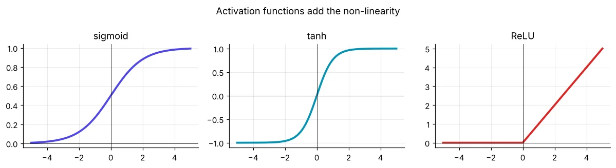
शुरू से neural network
समस्या: XOR – output 1 तब जब ठीक एक input 1 हो। कोई सीधी line इसे अलग नहीं कर सकती, इसलिए logistic regression fail होता है। एक hidden layer इसे हल करती है।
import numpy as np
rng = np.random.default_rng(1)
X = np.array([[0, 0], [0, 1], [1, 0], [1, 1]], dtype=float)
y = np.array([[0], [1], [1], [0]], dtype=float)
W1, b1 = rng.normal(0, 1, (2, 4)), np.zeros((1, 4))      # 2 inputs → 4 hidden neurons
W2, b2 = rng.normal(0, 1, (4, 1)), np.zeros((1, 1))      # 4 hidden → 1 output
sig = lambda z: 1 / (1 + np.exp(-z))
lr = 1.0
for epoch in range(5001):
    h = np.tanh(X @ W1 + b1)                  # forward pass
    out = sig(h @ W2 + b2)
    loss = np.mean((out - y) ** 2)
    d_out = 2 * (out - y) / len(X) * out * (1 - out)           # backpropagation
    d_h = d_out @ W2.T * (1 - h ** 2)
    W2 -= lr * h.T @ d_out; b2 -= lr * d_out.sum(0, keepdims=True)   # gradient descent step
    W1 -= lr * X.T @ d_h;   b1 -= lr * d_h.sum(0, keepdims=True)
    if epoch in (0, 500, 1000, 5000):
print(f"epoch {epoch:4d} loss {loss:.4f} predictions {out.ravel().round(2)}")- 1Forward: layer-दर-layer predictions
- 2Loss: कितना ग़लत, मापें
- 3Backward: chain rule हर weight का दोष बताता है
- 4Update: weight −= learning_rate × gradient
- 5कई epochs दोहराएँ
असली network: handwritten digits
import time
from sklearn.datasets import load_digits
from sklearn.model_selection import train_test_split
from sklearn.preprocessing import StandardScaler
from sklearn.pipeline import make_pipeline
from sklearn.neural_network import MLPClassifier
from sklearn.linear_model import LogisticRegression
X, y = load_digits(return_X_y=True)
X_tr, X_te, y_tr, y_te = train_test_split(X, y, test_size=0.25, random_state=0, stratify=y)
for name, clf in [("logistic regression", LogisticRegression(max_iter=3000)),
                  ("MLP 64-32", MLPClassifier(hidden_layer_sizes=(64, 32), max_iter=600, random_state=0))]:
    t = time.time(); m = make_pipeline(StandardScaler(), clf).fit(X_tr, y_tr)
print(f"{name:20s} test accuracy {m.score(X_te, y_te):.3f}")import matplotlib.pyplot as plt
from sklearn.datasets import load_digits
from sklearn.model_selection import train_test_split
from sklearn.preprocessing import StandardScaler
from sklearn.neural_network import MLPClassifier
X, y = load_digits(return_X_y=True)
X_tr, X_te, y_tr, y_te = train_test_split(X, y, test_size=0.25, random_state=0, stratify=y)
sc = StandardScaler().fit(X_tr)
mlp = MLPClassifier(hidden_layer_sizes=(64, 32), max_iter=600, early_stopping=True, random_state=0).fit(sc.transform(X_tr), y_tr)
fig, ax = plt.subplots(1, 2, figsize=(11, 3.6))
ax[0].plot(mlp.loss_curve_, color="#4f46e5", label="training loss")
ax2 = ax[0].twinx(); ax2.plot(mlp.validation_scores_, color="#16a34a", label="validation accuracy")
ax[0].set_xlabel("epoch"); ax[0].set_title("Loss falls, validation accuracy rises"); ax[0].legend(loc="center right"); ax2.legend(loc="lower right")
pred = mlp.predict(sc.transform(X_te)); wrong = (pred != y_te).nonzero()[0][:6]
for i, k in enumerate(wrong):
sub = fig.add_axes([0.55 + i * 0.07, 0.25, 0.065, 0.5]); sub.imshow(X_te[k].reshape(8, 8), cmap="gray_r"); sub.axis("off")
sub.set_title(f"{y_te[k]}→{pred[k]}", fontsize=9, color="#dc2626")
ax[1].axis("off"); ax[1].set_title("Mistakes (true → predicted)")
plt.show()
print(f"stopped after {mlp.n_iter_} epochs | test accuracy {mlp.score(sc.transform(X_te), y_te):.3f}")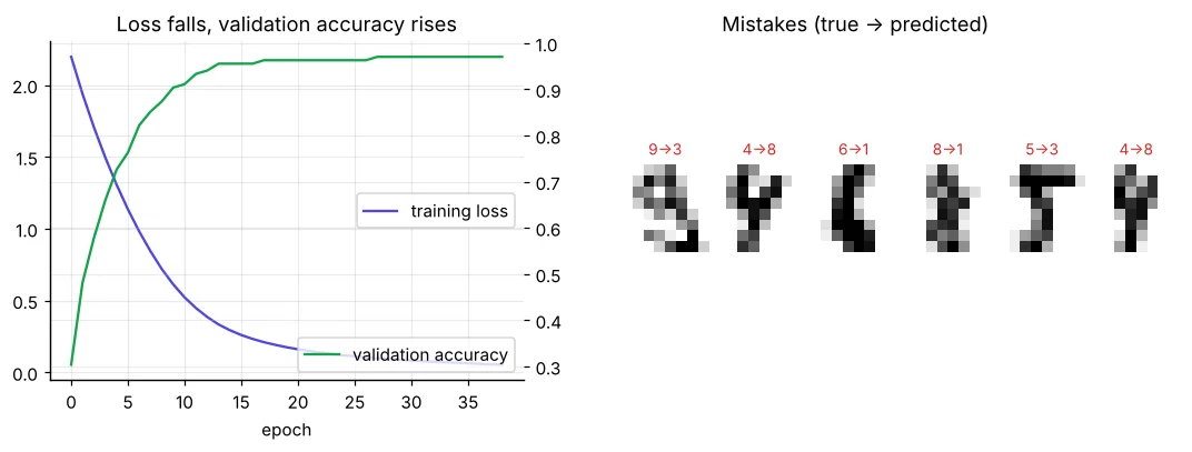
| Setting | क्या नियंत्रित करता है |
|---|---|
| hidden_layer_sizes | Network का आकार, जैसे (64, 32) = दो hidden layers |
| activation | "relu" (default), "tanh", "logistic" |
| learning_rate_init | Gradient descent का कदम |
| alpha | Overfitting के ख़िलाफ़ L2 regularisation |
| early_stopping | Validation सुधरना रुके तो रोकें |
| batch_size | हर weight update में rows |
Business tables पर neural nets
import pandas as pd
from sklearn.model_selection import cross_val_score
from sklearn.preprocessing import StandardScaler
from sklearn.pipeline import make_pipeline
from sklearn.neural_network import MLPClassifier
from sklearn.ensemble import HistGradientBoostingClassifier
from sklearn.linear_model import LogisticRegression
l = pd.read_csv("loan_applications.csv"); l["lti"] = l["loan_amount"] / (l["monthly_income"] * 12)
X, y = l[["monthly_income", "credit_score", "loan_amount", "years_employed", "lti"]], l["approved"]
for name, m in [("logistic", make_pipeline(StandardScaler(), LogisticRegression())),
                ("boosting", HistGradientBoostingClassifier(learning_rate=0.05, max_iter=200, random_state=0)),
                ("MLP 32-16", make_pipeline(StandardScaler(), MLPClassifier(hidden_layer_sizes=(32, 16), alpha=1e-2, max_iter=2000, random_state=0)))]:
print(f"{name:10s} CV AUC {cross_val_score(m, X, y, cv=5, scoring='roc_auc').mean():.3f}")छोटी tables पर simple models और boosting उतने ही या बेहतर – और समझाने में आसान। Deep learning images, audio, text और बहुत बड़े datasets पर जीतता है जहाँ यह features ख़ुद सीख सकता है।
Deep-learning परिवार
# pip install tensorflow   (needs more disk space; works on Google Colab out of the box)
import tensorflow as tf
from sklearn.datasets import load_digits
from sklearn.model_selection import train_test_split
X, y = load_digits(return_X_y=True)
X = X / 16.0
X_tr, X_te, y_tr, y_te = train_test_split(X, y, test_size=0.25, random_state=0, stratify=y)
model = tf.keras.Sequential([
    tf.keras.layers.Input(shape=(64,)),
    tf.keras.layers.Dense(64, activation="relu"),
    tf.keras.layers.Dropout(0.2),
    tf.keras.layers.Dense(32, activation="relu"),
    tf.keras.layers.Dense(10, activation="softmax"),
])
model.compile(optimizer="adam", loss="sparse_categorical_crossentropy", metrics=["accuracy"])
model.fit(X_tr, y_tr, epochs=30, batch_size=32, validation_split=0.1, verbose=0)
print(model.evaluate(X_te, y_te, verbose=0))
🏅 आज के Job Skills
Practice tasks
🏋️ Practice – ख़ुद करें
Solution देखें
import pandas as pd
from sklearn.model_selection import cross_val_score
from sklearn.pipeline import make_pipeline
from sklearn.compose import make_column_transformer
from sklearn.preprocessing import StandardScaler, OneHotEncoder
from sklearn.neural_network import MLPRegressor
from sklearn.linear_model import Ridge
h = pd.read_csv("house_prices.csv"); num = ["area_sqft", "bedrooms", "bathrooms", "age_years", "metro_km"]; cat = ["city", "furnishing", "parking"]
pre = make_column_transformer((StandardScaler(), num), (OneHotEncoder(), cat))
for name, m in [("Ridge", Ridge()), ("MLP", MLPRegressor(hidden_layer_sizes=(64, 32), max_iter=3000, random_state=0))]:
    s = -cross_val_score(make_pipeline(pre, m), h[num + cat], h["price_lakh"], cv=5, scoring="neg_mean_absolute_error")
print(name, round(s.mean(), 2))Quick quiz
🧠 Quick Quiz – ख़ुद को जाँचें
Interview corner
💼 Interview Corner
Backpropagation आसान शब्दों में समझाइए।
Forward pass के बाद loss मापते हैं; backpropagation chain rule से पीछे की ओर चलकर बताता है कि हर weight ने error में कितना योगदान दिया, फिर gradient descent हर weight को loss घटाने की दिशा में थोड़ा खिसकाता है।
Neural networks में overfitting कैसे रोकते हैं?
ज़्यादा data या augmentation, L2 regularisation (alpha / weight decay), dropout, validation set पर early stopping, छोटे networks, और pre-trained models से transfer learning।
सारांश
- Neuron = weighted sum + activation; layers neurons को जोड़ती हैं।
- Training = forward pass → loss → backprop → gradient step, बार-बार।
- MLPClassifier/MLPRegressor scikit-learn में neural nets देते हैं।
- Deep learning images, audio और text पर चमकता है; छोटी tables पर अक्सर boosting जीतता है।
Day 52: Analysts के लिए Excel और Power BI – वे tools जो हर business team पहले से इस्तेमाल करती है।